Class 3

R Basics, Files, and Projects

Materials for class on

2024-09-03

Agenda

Today we’re going to use some materials from a few different places, with a focus on:

Submitting to Gradescope (p3)
Babynames Data Analysis Demo/Walkthrough
Getting help (within R/RStudio)

Preparation Materials

Resources

Josef Fruehwald’s R Basics

Analyzing baby names

We need to load the packages we previously installed:

library(babynames)
library(tidyverse)

First we’ll try out some help, and then load and look at the included dataset:

help(babynames)
?babynames
help(package = "babynames")

data(babynames)
head(babynames)

#> # A tibble: 6 × 5
#>    year sex   name          n   prop
#>   <dbl> <chr> <chr>     <int>  <dbl>
#> 1  1880 F     Mary       7065 0.0724
#> 2  1880 F     Anna       2604 0.0267
#> 3  1880 F     Emma       2003 0.0205
#> 4  1880 F     Elizabeth  1939 0.0199
#> 5  1880 F     Minnie     1746 0.0179
#> 6  1880 F     Margaret   1578 0.0162

We can get a different type of preview with the glimpse() function.

glimpse(babynames)

#> Rows: 1,924,665
#> Columns: 5
#> $ year <dbl> 1880, 1880, 1880, 1880, 1880, 1880, 1880, 1880, 1880, 1880, 1880,…
#> $ sex  <chr> "F", "F", "F", "F", "F", "F", "F", "F", "F", "F", "F", "F", "F", …
#> $ name <chr> "Mary", "Anna", "Emma", "Elizabeth", "Minnie", "Margaret", "Ida",…
#> $ n    <int> 7065, 2604, 2003, 1939, 1746, 1578, 1472, 1414, 1320, 1288, 1258,…
#> $ prop <dbl> 0.07238359, 0.02667896, 0.02052149, 0.01986579, 0.01788843, 0.016…

glimpse() is part of the dplyr package, which is part of the tidyverse. You can specify that you want to use a function from a specific package by using two colons after the package name, like this:

dplyr::glimpse(babynames)

#> Rows: 1,924,665
#> Columns: 5
#> $ year <dbl> 1880, 1880, 1880, 1880, 1880, 1880, 1880, 1880, 1880, 1880, 1880,…
#> $ sex  <chr> "F", "F", "F", "F", "F", "F", "F", "F", "F", "F", "F", "F", "F", …
#> $ name <chr> "Mary", "Anna", "Emma", "Elizabeth", "Minnie", "Margaret", "Ida",…
#> $ n    <int> 7065, 2604, 2003, 1939, 1746, 1578, 1472, 1414, 1320, 1288, 1258,…
#> $ prop <dbl> 0.07238359, 0.02667896, 0.02052149, 0.01986579, 0.01788843, 0.016…

It does the same thing! This also lets you run a function without explicitly loading the package that it belongs to (such as running library(package).

The dplyr package has lots of useful tools for working with data. Another one is filter():

filter(babynames, name == "Lisa")

#> # A tibble: 159 × 5
#>     year sex   name      n      prop
#>    <dbl> <chr> <chr> <int>     <dbl>
#>  1  1886 F     Lisa      6 0.0000390
#>  2  1896 F     Lisa      5 0.0000198
#>  3  1899 F     Lisa      7 0.0000283
#>  4  1904 F     Lisa      9 0.0000308
#>  5  1905 F     Lisa      5 0.0000161
#>  6  1907 F     Lisa      7 0.0000207
#>  7  1910 F     Lisa      9 0.0000214
#>  8  1911 F     Lisa      9 0.0000204
#>  9  1912 F     Lisa      7 0.0000119
#> 10  1913 F     Lisa     16 0.0000244
#> # ℹ 149 more rows

Question

How many rows does the tibble have for your first name?

What does it mean if there are 0?

filter(babynames, name == "Lisa" & sex == "F")

#> # A tibble: 114 × 5
#>     year sex   name      n      prop
#>    <dbl> <chr> <chr> <int>     <dbl>
#>  1  1886 F     Lisa      6 0.0000390
#>  2  1896 F     Lisa      5 0.0000198
#>  3  1899 F     Lisa      7 0.0000283
#>  4  1904 F     Lisa      9 0.0000308
#>  5  1905 F     Lisa      5 0.0000161
#>  6  1907 F     Lisa      7 0.0000207
#>  7  1910 F     Lisa      9 0.0000214
#>  8  1911 F     Lisa      9 0.0000204
#>  9  1912 F     Lisa      7 0.0000119
#> 10  1913 F     Lisa     16 0.0000244
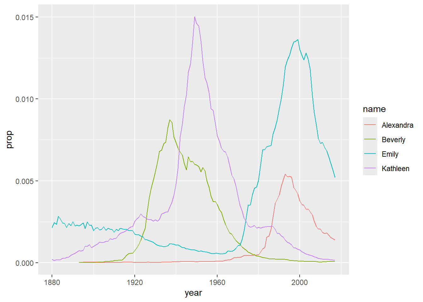
#> # ℹ 104 more rows

We can use this filtered data to make a plot:

ggplot(data = filter(babynames, name == "Lisa" & sex == "F"), mapping = aes(x = year,y = n))+
  geom_line()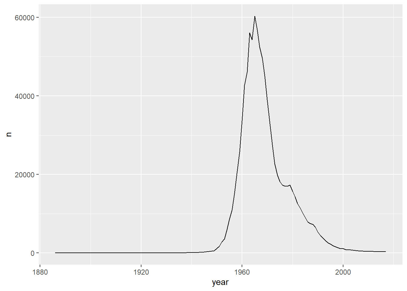

Try to make your own!

If we want to use multiple functions with the same data, the “pipe” is very useful. We will be seeing a lot of the R pipes - there are two “main” ones. The classic is called magrittr pipe as it is a part of the magrittr package, and is written %>%. There is a new one that is part of base R, |>. The magrittr pipe does more than the base R pipe, but for most purposes the base R version is fine.

Here are some examples of using the pipes:

babynames %>% 
  filter(.data = ., name == "Lisa" & year > 1999)

#> # A tibble: 19 × 5
#>     year sex   name      n       prop
#>    <dbl> <chr> <chr> <int>      <dbl>
#>  1  2000 F     Lisa   1087 0.000545  
#>  2  2000 M     Lisa      7 0.00000335
#>  3  2001 F     Lisa    908 0.000459  
#>  4  2002 F     Lisa    830 0.000420  
#>  5  2003 F     Lisa    811 0.000404  
#>  6  2004 F     Lisa    709 0.000352  
#>  7  2005 F     Lisa    618 0.000305  
#>  8  2006 F     Lisa    608 0.000291  
#>  9  2007 F     Lisa    524 0.000248  
#> 10  2008 F     Lisa    507 0.000244  
#> 11  2009 F     Lisa    420 0.000208  
#> 12  2010 F     Lisa    396 0.000202  
#> 13  2011 F     Lisa    396 0.000205  
#> 14  2012 F     Lisa    395 0.000204  
#> 15  2013 F     Lisa    353 0.000183  
#> 16  2014 F     Lisa    376 0.000193  
#> 17  2015 F     Lisa    373 0.000192  
#> 18  2016 F     Lisa    342 0.000177  
#> 19  2017 F     Lisa    305 0.000163

The pipe feeds the output of the previous line into the next function where the dot pronoun is specified. It works in this position because that is a data argument.

babynames %>% 
  filter(., name == "Lisa" & year > 1999)

#> # A tibble: 19 × 5
#>     year sex   name      n       prop
#>    <dbl> <chr> <chr> <int>      <dbl>
#>  1  2000 F     Lisa   1087 0.000545  
#>  2  2000 M     Lisa      7 0.00000335
#>  3  2001 F     Lisa    908 0.000459  
#>  4  2002 F     Lisa    830 0.000420  
#>  5  2003 F     Lisa    811 0.000404  
#>  6  2004 F     Lisa    709 0.000352  
#>  7  2005 F     Lisa    618 0.000305  
#>  8  2006 F     Lisa    608 0.000291  
#>  9  2007 F     Lisa    524 0.000248  
#> 10  2008 F     Lisa    507 0.000244  
#> 11  2009 F     Lisa    420 0.000208  
#> 12  2010 F     Lisa    396 0.000202  
#> 13  2011 F     Lisa    396 0.000205  
#> 14  2012 F     Lisa    395 0.000204  
#> 15  2013 F     Lisa    353 0.000183  
#> 16  2014 F     Lisa    376 0.000193  
#> 17  2015 F     Lisa    373 0.000192  
#> 18  2016 F     Lisa    342 0.000177  
#> 19  2017 F     Lisa    305 0.000163

babynames %>% 
  filter(name == "Lisa" & year > 1999)

#> # A tibble: 19 × 5
#>     year sex   name      n       prop
#>    <dbl> <chr> <chr> <int>      <dbl>
#>  1  2000 F     Lisa   1087 0.000545  
#>  2  2000 M     Lisa      7 0.00000335
#>  3  2001 F     Lisa    908 0.000459  
#>  4  2002 F     Lisa    830 0.000420  
#>  5  2003 F     Lisa    811 0.000404  
#>  6  2004 F     Lisa    709 0.000352  
#>  7  2005 F     Lisa    618 0.000305  
#>  8  2006 F     Lisa    608 0.000291  
#>  9  2007 F     Lisa    524 0.000248  
#> 10  2008 F     Lisa    507 0.000244  
#> 11  2009 F     Lisa    420 0.000208  
#> 12  2010 F     Lisa    396 0.000202  
#> 13  2011 F     Lisa    396 0.000205  
#> 14  2012 F     Lisa    395 0.000204  
#> 15  2013 F     Lisa    353 0.000183  
#> 16  2014 F     Lisa    376 0.000193  
#> 17  2015 F     Lisa    373 0.000192  
#> 18  2016 F     Lisa    342 0.000177  
#> 19  2017 F     Lisa    305 0.000163

The base R pipe doesn’t have a dot pronoun, so it works only in the default position:

babynames |> 
  filter(name == "Lisa" & year > 1999)

#> # A tibble: 19 × 5
#>     year sex   name      n       prop
#>    <dbl> <chr> <chr> <int>      <dbl>
#>  1  2000 F     Lisa   1087 0.000545  
#>  2  2000 M     Lisa      7 0.00000335
#>  3  2001 F     Lisa    908 0.000459  
#>  4  2002 F     Lisa    830 0.000420  
#>  5  2003 F     Lisa    811 0.000404  
#>  6  2004 F     Lisa    709 0.000352  
#>  7  2005 F     Lisa    618 0.000305  
#>  8  2006 F     Lisa    608 0.000291  
#>  9  2007 F     Lisa    524 0.000248  
#> 10  2008 F     Lisa    507 0.000244  
#> 11  2009 F     Lisa    420 0.000208  
#> 12  2010 F     Lisa    396 0.000202  
#> 13  2011 F     Lisa    396 0.000205  
#> 14  2012 F     Lisa    395 0.000204  
#> 15  2013 F     Lisa    353 0.000183  
#> 16  2014 F     Lisa    376 0.000193  
#> 17  2015 F     Lisa    373 0.000192  
#> 18  2016 F     Lisa    342 0.000177  
#> 19  2017 F     Lisa    305 0.000163

We can string together many functions with pipes:

babynames |> 
  group_by(name, sex) |> 
  count() |>
  group_by(name) |> 
  count() |> 
  filter(n == 2)

#> # A tibble: 10,663 × 2
#> # Groups:   name [10,663]
#>    name        n
#>    <chr>   <int>
#>  1 Aaden       2
#>  2 Aadi        2
#>  3 Aadyn       2
#>  4 Aalijah     2
#>  5 Aaliyah     2
#>  6 Aaliyan     2
#>  7 Aamari      2
#>  8 Aamir       2
#>  9 Aaren       2
#> 10 Aareon      2
#> # ℹ 10,653 more rows

If we want to “keep” what we’ve done, we have to use assignment:

df_bothMF <- babynames |>
  group_by(name, sex) |> 
  count() |>
  group_by(name) |> 
  count() |>
  filter(n == 2)

df_somenames <- babynames |> 
  filter(name %in% c("Emily","Kathleen","Alexandra","Beverly"), sex=="F") 

ggplot(data = df_somenames, mapping = aes(x = year,y = prop, color=name))+
  geom_line()