Dataframes and tibbles are kinds of tables, and in R tables are really a set of vectors! Sets of vectors are formally known as “lists” in R, but you don’t really need to really know all of the things that lists do to work with them and understand them.
Subsetting Dataframes
You’ve already seen a bit of tidyverse subsetting of data with filter(), but let’s look at some base R techniques.
If you want to extract just one column/variable vector with base R, you can use the $ operator. Let’s use the built-in starwars dataset:
With dataframes (and other lists) we can also use bracket subsetting, but we now have two dimensions - rows and columns. We can subset by row, by column, or by both. Row is first, then column (like “RC Cola” if you’ve heard of it!), the same as matrix indexing if you’re familiar.
# dataframe[row, column]# only row 1, column 1starwars[1,1]
#> # A tibble: 1 × 1
#>   name
#>   <chr>
#> 1 Luke Skywalker
# all rows, but only column 1starwars[,1]
#> # A tibble: 87 × 1
#>    name
#>    <chr>
#>  1 Luke Skywalker
#>  2 C-3PO
#>  3 R2-D2
#>  4 Darth Vader
#>  5 Leia Organa
#>  6 Owen Lars
#>  7 Beru Whitesun Lars
#>  8 R5-D4
#>  9 Biggs Darklighter
#> 10 Obi-Wan Kenobi
#> # ℹ 77 more rows
# only row 1, all columnsstarwars[1,]
#> # A tibble: 1 × 14
#>   name      height  mass hair_color skin_color eye_color birth_year sex   gender
#>   <chr>      <int> <dbl> <chr>      <chr>      <chr>          <dbl> <chr> <chr>
#> 1 Luke Sky…    172    77 blond      fair       blue              19 male  mascu…
#> # ℹ 5 more variables: homeworld <chr>, species <chr>, films <list>,
#> #   vehicles <list>, starships <list>
You can use logical expressions in the brackets in the same way as in vector subsetting.
There is also a [[ subsetting operator, but we don’t need it for now.
Question
How would you do something similar to starwars[1,] with a tidyverse function you know?
Question
What about starwars[,1]?
This page may be helpful for some base R and tidyverse translations.
There are some other tidyverse functions we haven’t encountered yet that do similar work, such as pull() and slice().
Recyclying
Some functions permit recycling of vectors, and the rules for it vary depending on the function. One of the tidyverse constraints imposes a limit to recycling so that it’s only permitted for 1-element vectors, but many base R functions allow more complex recycling. What is recycling? Let’s look at an example.
a <-1:10b <-5
b is a vector with one element. In vector operations, it can be “recycled” to match the length of a longer vector, as long as the longer one is divisible by the length of the shorter one (here 10 is divisible by 1).
c <- a * bc
#> [1] 5 10 15 20 25 30 35 40 45 50
for (i in a){ c <- a * b}c
#> [1] 5 10 15 20 25 30 35 40 45 50
If we have a vector with two elements, it will also recycle, but 5 times, cycling through the shorter vector:
d <-c(1, 100) # 2-element vectora * d
#> [1] 1 200 3 400 5 600 7 800 9 1000
If we have vectors of length 3 and 10, recycling will throw a warning because 10 is not a multiple of 3:
e <-c(1, 10, 100) # 3-element vectora * e
#> Warning in a * e: longer object length is not a multiple of shorter object
#> length
#> [1] 1 20 300 4 50 600 7 80 900 10
Data Visualization
Poll
Are you colorblind (to any degree)?
yes
no
5-8% of folks with xy chromosomes are! Much smaller proportion for xx and other folks. You may want to check out the Pebble-Safe colorblind-friendly Rstudio themes. There are many resources for more accessible data viz, including color accessibility. Some are linked on our Resources page. There is no completely automated way to make sure your visualizations are accessible to everyone, so it’s important to be mindful of.
Interactive Work
The main thing we want to get comfortable with here is thinking about how data relates to visualization, and how that translates into ggplot2 code in the spirit of the “grammar of graphics”.
We’ll work through some ggplot basics and exercises “interactively” during class and I’ll share the results back to the Google Drive after class. So this is just a sketch of topics for now! Open up your p4 assignment file so you can compare your answers and add some more examples.
ggplot fundamentals
library(tidyverse)data(diamonds)diamonds
#> # A tibble: 53,940 × 10
#>    carat cut       color clarity depth table price     x     y     z
#>    <dbl> <ord>     <ord> <ord>   <dbl> <dbl> <int> <dbl> <dbl> <dbl>
#>  1  0.23 Ideal     E     SI2      61.5    55   326  3.95  3.98  2.43
#>  2  0.21 Premium   E     SI1      59.8    61   326  3.89  3.84  2.31
#>  3  0.23 Good      E     VS1      56.9    65   327  4.05  4.07  2.31
#>  4  0.29 Premium   I     VS2      62.4    58   334  4.2   4.23  2.63
#>  5  0.31 Good      J     SI2      63.3    58   335  4.34  4.35  2.75
#>  6  0.24 Very Good J     VVS2     62.8    57   336  3.94  3.96  2.48
#>  7  0.24 Very Good I     VVS1     62.3    57   336  3.95  3.98  2.47
#>  8  0.26 Very Good H     SI1      61.9    55   337  4.07  4.11  2.53
#>  9  0.22 Fair      E     VS2      65.1    61   337  3.87  3.78  2.49
#> 10  0.23 Very Good H     VS1      59.4    61   338  4     4.05  2.39
#> # ℹ 53,930 more rows
Let’s build up a plot one piece at a time.
Question
How would you tell ggplot() what data you want to plot from, and nothing else?
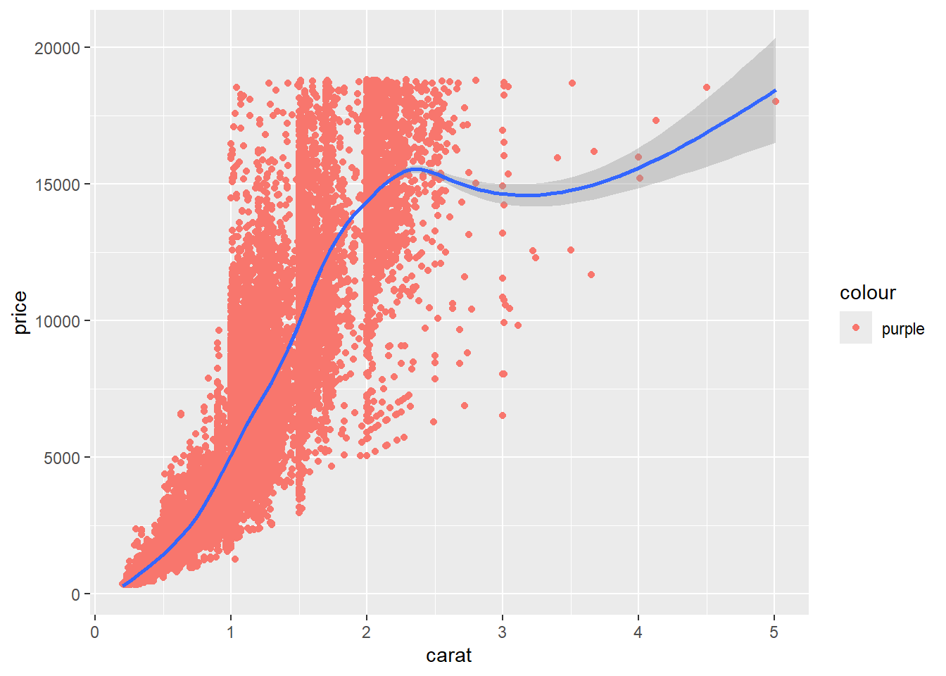
difference between color and color aesthetic!
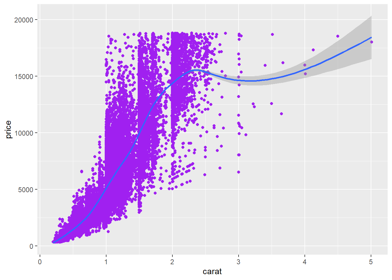
You can specify global aesthetics for the whole plot, or ones that are specific to only one geom (local). Local aesthetics will override global ones for that geom. You can set a global aesthetic outside of the initial ggplot() function, but it will only apply to subsequent layers/geoms.
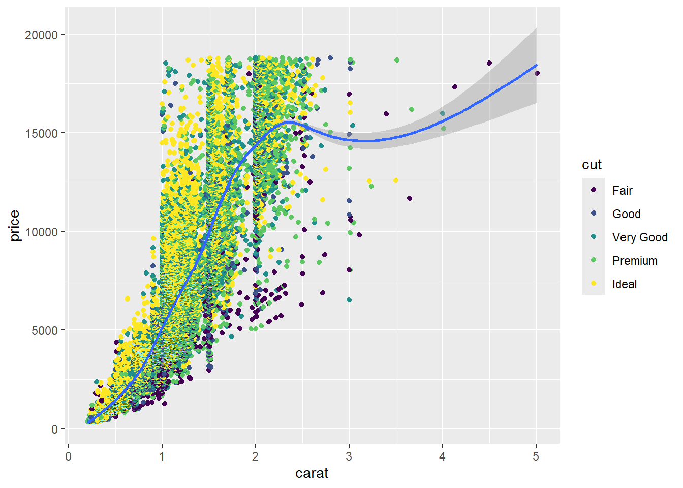
Change color with the “cut” variable in a geom-specific aes() call:
#> `geom_smooth()` using method = 'gam' and formula = 'y ~ s(x, bs = "cs")'
Source Code
---title: "Class 5"subtitle: "Basics Continued and Data Visualization"date: 2024-09-10date-format: "YYYY-MM-DD"editor: markdown: wrap: 72editor_options: chunk_output_type: console---## Preparation Materials- {{< fa external-link >}} [Data Visualization (R for Data Science 2e)](https://r4ds.hadley.nz/data-visualize.html)## AgendaToday we'll focus on:- R programming basics continued (dataframes)- What really is a function? A package?- p4 review/questions (data visualization)- p5 start - summarize and create your own viz## DataframesDataframes and tibbles are kinds of tables, and in R tables are really a set of vectors! Sets of vectors are formally known as "lists" in R, but youdon't really need to really know all of the things that lists do to work with them and understand them. ### Subsetting DataframesYou've already seen a bit of tidyverse subsetting of data with `filter()`, butlet's look at some base R techniques.If you want to extract just one column/variable vector with base R, you canuse the `$` operator. Let's use the built-in `starwars` dataset:```{r}library(tidyverse)starwars$name```With dataframes (and other lists) we can also use bracket subsetting, butwe now have two dimensions - rows and columns. We can subset by row, by column,or by both. Row is first, then column (like "RC Cola" if you've heard of it!), the same as matrix indexing if you're familiar. ```{r}# dataframe[row, column]# only row 1, column 1starwars[1,1]# all rows, but only column 1starwars[,1]# only row 1, all columnsstarwars[1,]```You can use logical expressions in the brackets in the same way as in vectorsubsetting. There is also a `[[` subsetting operator, but we don't need it for now. ::: {.callout-note .question}## QuestionHow would you do something similar to `starwars[1,]` with a tidyversefunction you know?:::::: {.callout-note .question}## QuestionWhat about `starwars[,1]`?:::[This page](https://dplyr.tidyverse.org/articles/base.html) may be helpful for some base R and tidyverse translations. There are some other tidyverse functions we haven't encountered yet that do similar work, such as `pull()` and `slice()`. ## RecyclyingSome functions permit recycling of vectors, and the rules for it varydepending on the function. One of the tidyverse constraints imposes alimit to recycling so that it's only permitted for 1-element vectors,but many base R functions allow more complex recycling. What isrecycling? Let's look at an example.```{r}a <-1:10b <-5````b` is a vector with one element. In vector operations, it can be"recycled" to match the length of a longer vector, as long as the longerone is divisible by the length of the shorter one (here 10 is divisibleby 1).```{r vector3}c <- a * bc``````{r loop3}for (i in a){ c <- a * b}c```If we have a vector with two elements, it will also recycle, but 5times, cycling through the shorter vector:```{r}d <-c(1, 100) # 2-element vectora * d```If we have vectors of length 3 and 10, recycling will throw a warningbecause 10 is not a multiple of 3:```{r, error = TRUE}e <- c(1, 10, 100) # 3-element vectora * e```## Data Visualization::: {.callout-note .question}## PollAre you colorblind (to any degree)? (a) yes (b) no::: 5-8% of folks with xy chromosomes are! Much smaller proportion for xx and other folks. You may want to check out the [Pebble-Safe colorblind-friendly Rstudio themes](https://github.com/DesiQuintans/Pebble-safe).There are many resources for more accessible data viz, includingcolor accessibility. Some are linked on our [Resources](/resources.qmd) page. There is no completely automated way to make sure your visualizations are accessible to everyone, so it's important to be mindful of. ## Interactive WorkThe main thing we want to get comfortable with here is thinking about howdata relates to visualization, and how that translates into `ggplot2` codein the spirit of the "grammar of graphics". We'll work through some ggplot basics and exercises "interactively" during class and I'll share the results back to the Google Drive after class. So this is just a sketch of topics for now! **Open up your p4 assignment file** so you can compare your answers and add some more examples.## ggplot fundamentals```{r}library(tidyverse)data(diamonds)diamonds```Let's build up a plot one piece at a time. ::: {.callout-note .question}## QuestionHow would you tell `ggplot()` what data you want to plot from, and nothing else?:::### difference between color and color aesthetic!You can specify global aesthetics for the whole plot, or ones thatare specific to only one geom (local). Local aesthetics will override global ones for that geom. You can set a global aestheticoutside of the initial `ggplot()` function, but it will only applyto subsequent layers/geoms. Change color with the "cut" variable in a geom-specific `aes()` call:```{r}ggplot(diamonds, mapping =aes(x = carat, y = price)) +geom_point(aes(color = cut)) +geom_smooth()```What happens if you try to set an aesthetic to a color rather than a variable?```{r}ggplot(diamonds, mapping =aes(x = carat, y = price)) +geom_point(aes(color ="purple")) +geom_smooth()```::: {.callout-note .question}## QuestionWhy are all of the points the same "salmon" color now? Nothing is purple? (a) yes (b) no::: Let's take the color specification outside of the aesthetics. That's better!(If what you want is all blue dots)```{r}ggplot(diamonds, mapping =aes(x = carat, y = price)) +geom_point(color ="purple") +geom_smooth()```