#> [1] 482Class 6
Quarto Reports and Review
Agenda
Today we’ll focus on:
- What are functions?
- Creating and rendering Quarto html reports
What are functions?
Just briefly to demystify a bit - what are these functions we’re using?
Most of them are just pre-built sets of R code for a particular purpose. Someone has combined a bunch of code for you so that you don’t have to think through all of the steps.
You can write your own functions. Here’s a somewhat silly example:
Question
Try to create a function that would multiply three numbers.
The type of functions is “closure”. You may encounter this term in an error one day - tuck it away in your brain somewhere!
Packages are collections of such functions, documentation, and sometimes data that others have put together in a format that is easy to share with others. You can even create your own package of personal functions - this is not necessary for doing data analysis, but I will provide pointers to doing this later in the semester.
Quarto: Interactive Work
We’ll work through creating Quarto reports in class, and I will share the output on Google Drive so that you can see it as a document outside of the style of this website, which will look more like your own Quarto documents.
Some examples of what Quarto is for: https://quarto.org/docs/gallery/
You can use Quarto with different IDEs, but the Quarto tutorial for RStudio begins here: https://quarto.org/docs/get-started/hello/rstudio.html
You should already have Quarto installed if you followed the instructions for installing the most recent version of RStudio, which is “bundled” with Quarto.
You can use Quarto with other languages like Python, but we will focus on just R to start.
This is the HTML authoring page which should have most of the information you need to reference for that type of report.
R Sessions in Quarto and R Markdown
When you knit or render reports, they will start (and end) a new R session. This means that you need to make sure that all packages and objects are made accessible through lines of code in the report, and not through the console or other scripts prior to knitting/rendering. If packages/objects are “not found” this is the most likely culprit!
Creating your Quarto Doc and Rendering
While in your class project (or starting a new project), create a new Quarto file, set to render html using knitr. Name your file with today’s class or date and your last name, without any spaces.
You should get a default Quarto template. Test rendering by clicking the Render button. You should see an html file in your project folder which has the same filename as the original Quarto document, but ending with .html, for example class6.html. This is your output. It may also create a new folder (depending on what was in your document).
Render Often
When working with Quarto, you don’t need to render, you can just run the script interatively like an R script. However, if you do plan to share the rendered output, it is good practice to test rendering somewhat frequently. This makes it easier to identify where any rendering errors might be coming from (presumably only your most recent changes!).
Code Output Customization
When you work with a document like Quarto, you have choices about where you want your code output to appear. You can adjust this in your YAML header, with editor_options and the chunk_output_type. If you choose console, the output will show in the console, similar to running lines interactively in a .R script. If you choose inline, the output will appear in the pane with your code. I personally prefer console to keep my script separate from output, and also to prevent my editor pane from “jumping around” and pushing the next code chunk further away whenever output fills in the pane space!
Simplifying HTML output for sharing
When creating an html document with Quarto, images will be generated if you have plots. By default, these are saved in a folder. If you want to share the files with others without web hosting, you need to either include this folder, or you can instead render them as “self-contained” or “standalone” which will embed the images into one file. To make a standalone html document, add that to your YAML header:
Summarization and Plotting Practice: Interactive Work
I will answer questions that have already come up with your practice work, but here are some more exercises to try. I’m giving you the answers - you find the code to generate those answers! We will share some to iClicker.
Do all of the following work in a new Quarto file for today.
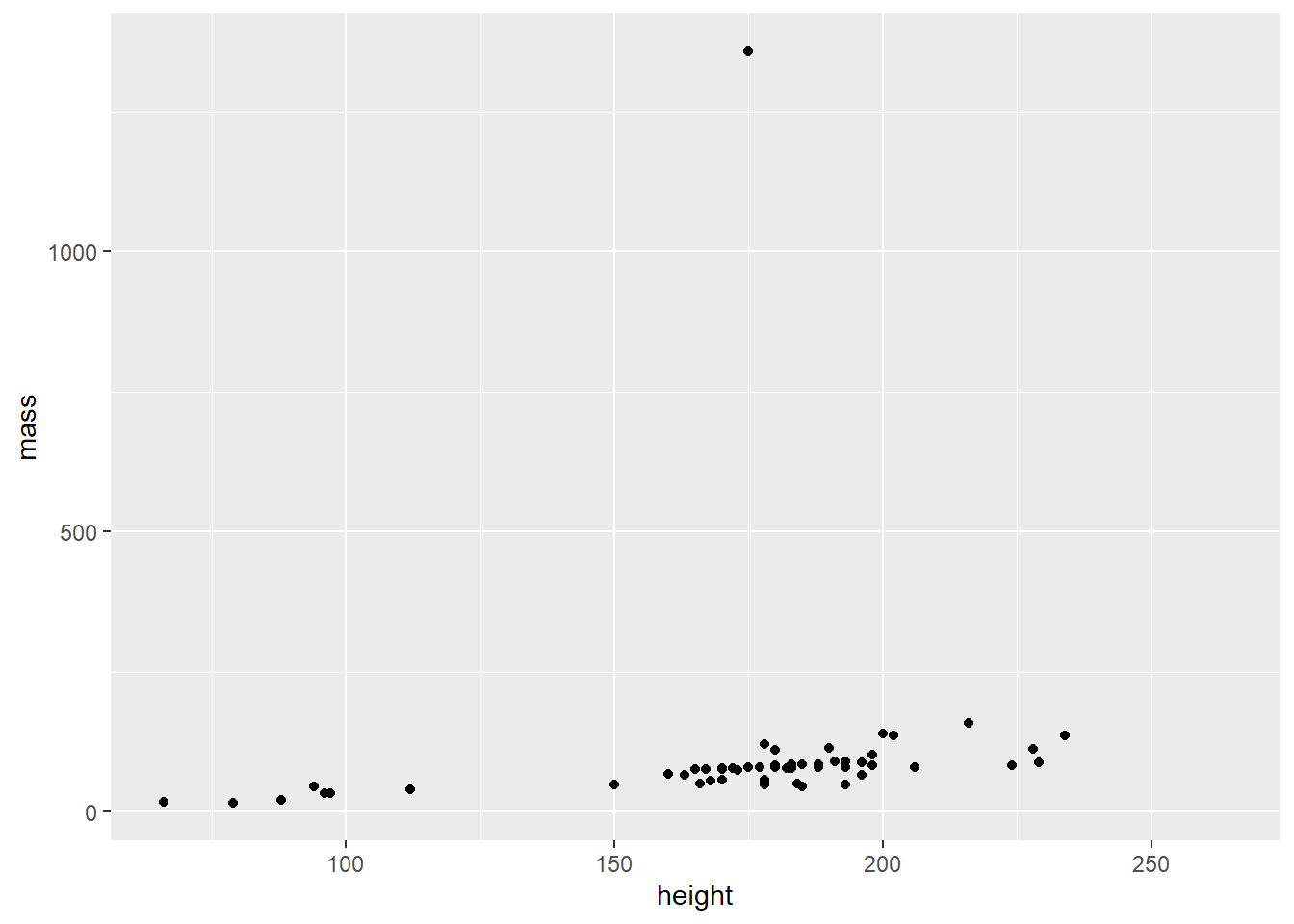
- Use the
starwarsdataset to create the following plot:
- Modify the underlying data so that we can focus on most of the values:
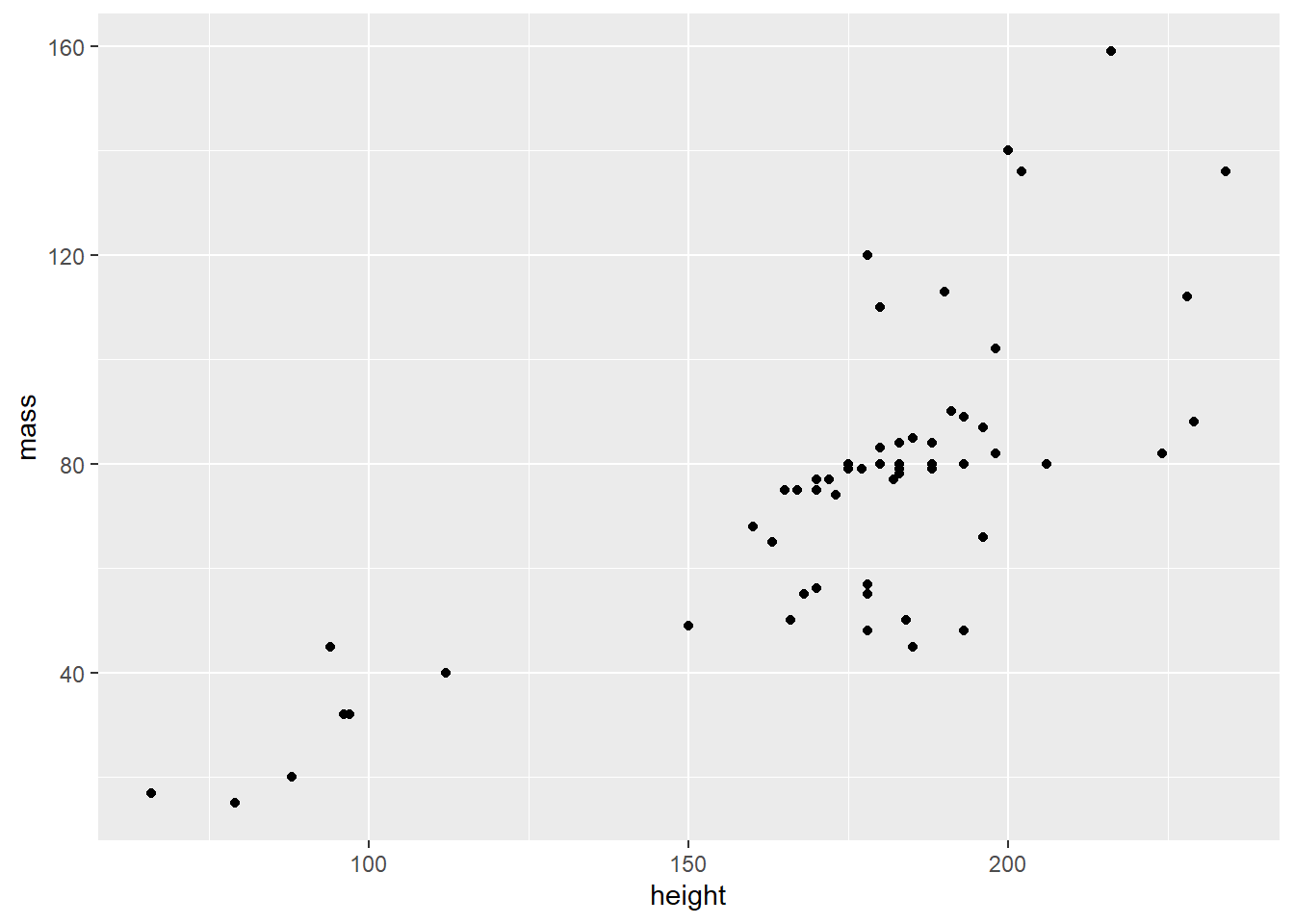
- Create a regression line that shows the relationship between height and mass. Use the “lm” (linear model) method:
starwars |>
  filter(mass < 1000) |>
  ggplot(aes(x = height, y = mass)) +
geom_point() +
geom_smooth(method = "lm")#> `geom_smooth()` using formula = 'y ~ x'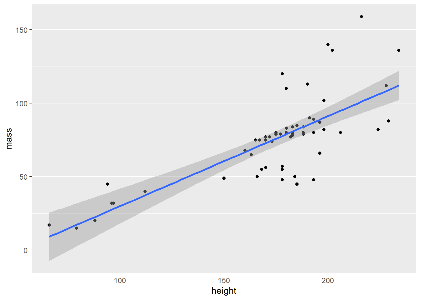
- Let’s see if there is any difference in the slope of the line for gender. But you’ll need to remove any data with
NA(missing) gender.
starwars |>
  filter(mass < 1000 & !is.na(gender)) |>
  ggplot(aes(x = height, y = mass, color = gender)) +
  geom_point() +
  geom_smooth(method = "lm")
#> `geom_smooth()` using formula = 'y ~ x'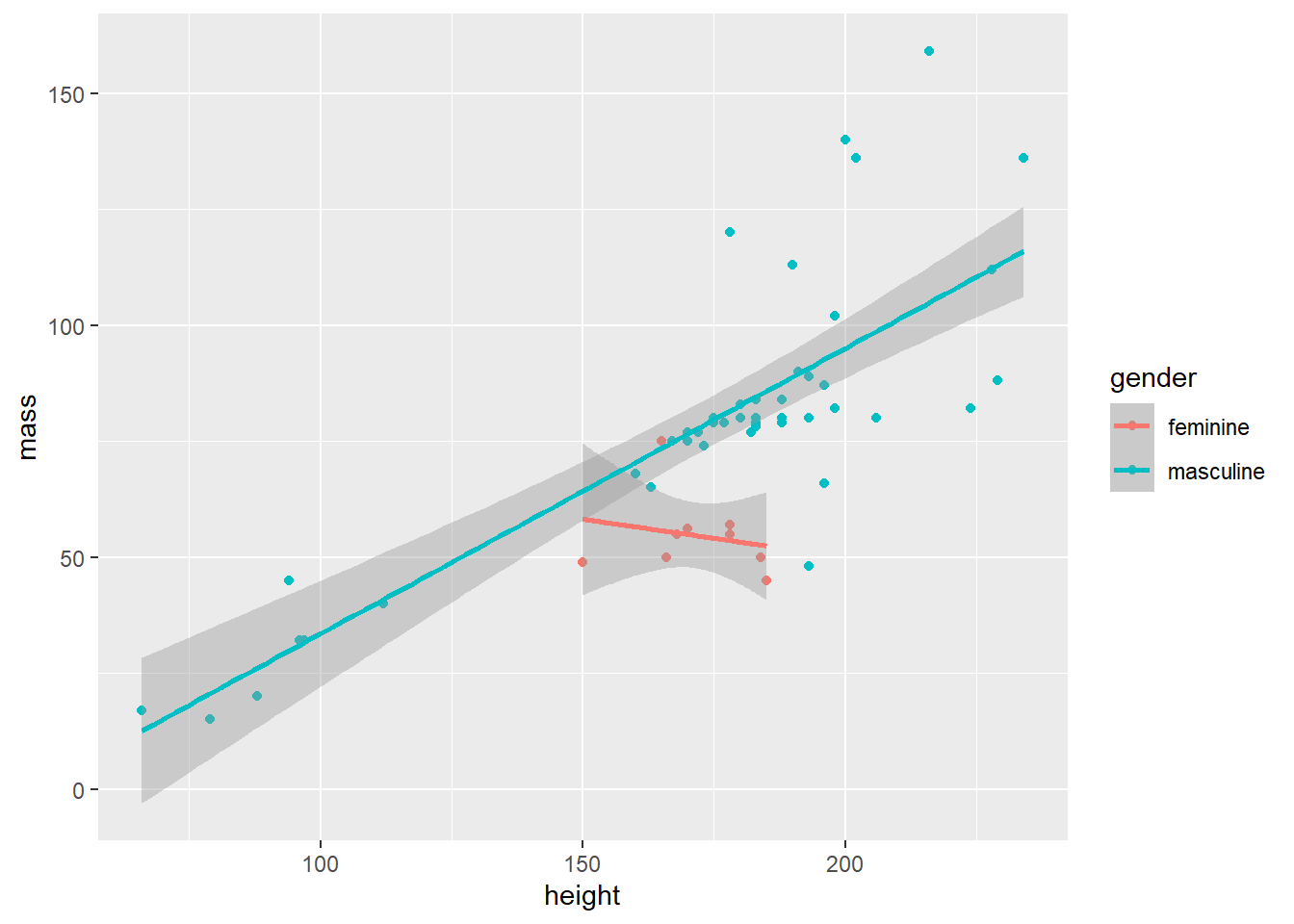
- What is the average (mean) height for each species?
#> # A tibble: 38 × 2
#> species mean_height
#> <chr> <dbl>
#> 1 Aleena 79
#> 2 Besalisk 198
#> 3 Cerean 198
#> 4 Chagrian 196
#> 5 Clawdite 168
#> 6 Droid 131.
#> 7 Dug 112
#> 8 Ewok 88
#> 9 Geonosian 183
#> 10 Gungan 209.
#> # ℹ 28 more rows- Which species the 3 highest and 3 lowest mean heights? HINT: use
slice_max()andslice_min(), and the help if needed.
starwars |>
  group_by(species) |>
summarize(mean_height = mean(height, na.rm = TRUE)) |>
slice_min(mean_height, n=3)#> # A tibble: 3 × 2
#> species mean_height
#> <chr> <dbl>
#> 1 Yoda's species 66
#> 2 Aleena 79
#> 3 Ewok 88starwars |>
group_by(species) |>
summarize(mean_height = mean(height, na.rm = TRUE)) |>
slice_max(mean_height, n=3)#> # A tibble: 3 × 2
#> species mean_height
#> <chr> <dbl>
#> 1 Quermian 264
#> 2 Wookiee 231
#> 3 Kaminoan 221- Create a new column that converts the height in cm to height in inches, by dividing by 2.54.
#> # A tibble: 87 × 15
#>    name     height  mass hair_color skin_color eye_color birth_year sex   gender
#>    <chr>     <int> <dbl> <chr>      <chr>      <chr>          <dbl> <chr> <chr>
#>  1 Luke Sk…    172    77 blond      fair       blue            19   male  mascu…
#>  2 C-3PO       167    75 <NA>       gold       yellow         112   none  mascu…
#>  3 R2-D2        96    32 <NA>       white, bl… red             33   none  mascu…
#>  4 Darth V…    202   136 none       white      yellow          41.9 male  mascu…
#>  5 Leia Or…    150    49 brown      light      brown           19   fema… femin…
#>  6 Owen La…    178   120 brown, gr… light      blue            52   male  mascu…
#>  7 Beru Wh…    165    75 brown      light      blue            47   fema… femin…
#>  8 R5-D4        97    32 <NA>       white, red red             NA   none  mascu…
#>  9 Biggs D…    183    84 black      light      brown           24   male  mascu…
#> 10 Obi-Wan…    182    77 auburn, w… fair       blue-gray       57   male  mascu…
#> # ℹ 77 more rows
#> # ℹ 6 more variables: homeworld <chr>, species <chr>, films <list>,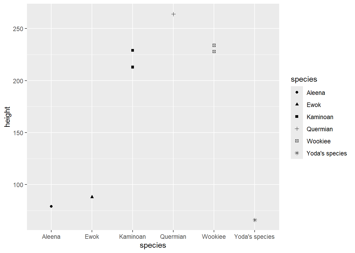
#> # vehicles <list>, starships <list>, height_inches <dbl>- Plot the heights of the individuals in these species like so:
starwars |>
  filter(species %in% c("Yoda's species", "Aleena", "Ewok", "Quermian", "Wookiee", "Kaminoan")) |>
  ggplot(aes(x = species, y = height)) +
  geom_point()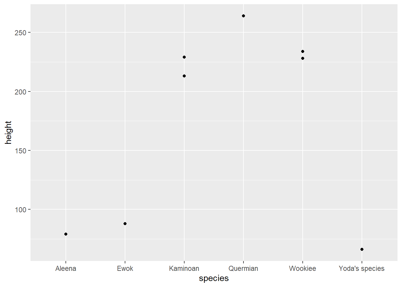
- Make the points different shapes for each species: