Class 11
Experiment Analsyis and Joins
Preparation Materials
Agenda
Today we’ll focus on:
- follow-up from last week
- joins!
- Quarto chunk option tips (help with prep assignment)
Before we get into it, let’s see how Hadley Wickham, founder of the tidyverse and Chief Scientist at Posit (maker of RStudio), handles some data analysis challenges, in his TidyTuesday screencast about cocktails.
Continuing Experimental Data Analysis
Let’s return to our experimental data analysis. Go back to the same project, or if you are starting from scratch, make sure to run the following to load the data in the same way:
- Setup the code to use
here:
- Use
here()with a relative path to load the data:
df <- read.csv(here("data", "delong maze 40Ss.csv"),
              header = 1,
              sep = ",",
              comment.char = "#",
              strip.white = T,
col.names = c("Index","Time","Counter","Hash","Owner","Controller","Item","Element","Type","Group","FieldName","Value","WordNum","Word","Alt","WordOn","CorrWord","RT","Sent","TotalTime","Question","Resp","Acc","RespRT"))- Create a new dataframe with only the rows that have the value “Maze” for the
Controllervariable, and don’t have the word “practice” inType.
- Take everything in
Typein the remaining data, and useseparate_wider_delim()to make separate columns from all of the variable names separated by periods (.).
# for auto naming, use names_sep
df_maze |>
  separate_wider_delim(cols = Type, delim = ".", names_sep = "")
#> # A tibble: 70,122 × 31
#> Index Time Counter Hash Owner Controller Item Element Type1 Type2 Type3
#> <int> <chr> <int> <chr> <chr> <chr> <int> <int> <chr> <chr> <chr>
#> 1 0 2021-03… 4 U+8f… no Maze 86 0 delo… 38 unex…
#> 2 0 2021-03… 4 U+8f… no Maze 86 0 delo… 38 unex…
#> 3 0 2021-03… 4 U+8f… no Maze 86 0 delo… 38 unex…
#> 4 0 2021-03… 4 U+8f… no Maze 86 0 delo… 38 unex…
#> 5 0 2021-03… 4 U+8f… no Maze 86 0 delo… 38 unex…
#> 6 0 2021-03… 4 U+8f… no Maze 86 0 delo… 38 unex…
#> 7 0 2021-03… 4 U+8f… no Maze 86 0 delo… 38 unex…
#> 8 0 2021-03… 4 U+8f… no Maze 86 0 delo… 38 unex…
#> 9 0 2021-03… 4 U+8f… no Maze 86 0 delo… 38 unex…
#> 10 0 2021-03… 4 U+8f… no Maze 86 0 delo… 38 unex…
#> # ℹ 70,112 more rows
#> # ℹ 20 more variables: Type4 <chr>, Type5 <chr>, Type6 <chr>, Type7 <chr>,
#> # Type8 <chr>, Group <chr>, FieldName <chr>, Value <chr>, WordNum <int>,
#> # Word <chr>, Alt <chr>, WordOn <int>, CorrWord <chr>, RT <int>, Sent <chr>,
#> # TotalTime <int>, Question <chr>, Resp <chr>, Acc <int>, RespRT <int>Let’s remove some extra/confusing columns:
df_maze <- df_maze |>
  select(Index, exp, item_num, expect, position, art.cloze, n.cloze, WordNum, Word, Alt, WordOn, CorrWord, RT, Sent)
df_maze
#> # A tibble: 70,122 × 14
#> Index exp item_num expect position art.cloze n.cloze WordNum Word Alt
#> <int> <chr> <chr> <chr> <chr> <chr> <chr> <int> <chr> <chr>
#> 1 0 delong 38 unexpec… 15 0 0 0 When x-x-x
#> 2 0 delong 38 unexpec… 15 0 0 1 the cent
#> 3 0 delong 38 unexpec… 15 0 0 2 pipe rely
#> 4 0 delong 38 unexpec… 15 0 0 3 broke weird
#> 5 0 delong 38 unexpec… 15 0 0 4 in sure
#> 6 0 delong 38 unexpec… 15 0 0 5 the glad
#> 7 0 delong 38 unexpec… 15 0 0 6 bath… anyw…
#> 8 0 delong 38 unexpec… 15 0 0 7 Feli… Deci…
#> 9 0 delong 38 unexpec… 15 0 0 8 look… summ…
#> 10 0 delong 38 unexpec… 15 0 0 9 thro… cult…
#> # ℹ 70,112 more rows
#> # ℹ 4 more variables: WordOn <int>, CorrWord <chr>, RT <int>, Sent <chr>- Let’s find the demographic data so we can use it in our analysis.
Pivot the demographic data wider so that the
FieldNamebecomes the names of new columns andValuehas the observations. Do you get the right number of rows? There are 39 participants in the experiment.Join the demographic data with the maze data so that each row has a variable for the participant’s age.
Create a new column called
sideto indicate in characters whether the real word was on the left or right, based on theWordOnvariable where 0 is left, 1 is right. Changeageto be numeric.Filter to rows where
WordNumis the same asposition- these are the rows with data for the “critical” position in the experiment, where the expected or unexpected noun would be.Summarize the reaction times with a mean, grouped by expectation. Which took longer?
Did all participants take longer for unexpected nouns?
Did older participants have longer reaction times?
Join By Notes
For joins, there is a new way to specify which variables to join by. Details here.
The old way is still possible, but there is a new option. Here are the two versions:
Original:
#> # A tibble: 336,776 × 27
#>    year.x month   day dep_time sched_dep_time dep_delay arr_time sched_arr_time
#>     <int> <int> <int>    <int>          <int>     <dbl>    <int>          <int>
#>  1   2013     1     1      517            515         2      830            819
#>  2   2013     1     1      533            529         4      850            830
#>  3   2013     1     1      542            540         2      923            850
#>  4   2013     1     1      544            545        -1     1004           1022
#>  5   2013     1     1      554            600        -6      812            837
#>  6   2013     1     1      554            558        -4      740            728
#>  7   2013     1     1      555            600        -5      913            854
#>  8   2013     1     1      557            600        -3      709            723
#>  9   2013     1     1      557            600        -3      838            846
#> 10   2013     1     1      558            600        -2      753            745
#> # ℹ 336,766 more rows
#> # ℹ 19 more variables: arr_delay <dbl>, carrier <chr>, flight <int>,
#> #   tailnum <chr>, origin <chr>, dest <chr>, air_time <dbl>, distance <dbl>,
#> #   hour <dbl>, minute <dbl>, time_hour <dttm>, year.y <int>, type <chr>,
#> #   manufacturer <chr>, model <chr>, engines <int>, seats <int>, speed <int>,
#> # engine <chr>#> # A tibble: 336,776 × 27
#> year.x month day dep_time sched_dep_time dep_delay arr_time sched_arr_time
#> <int> <int> <int> <int> <int> <dbl> <int> <int>
#> 1 2013 1 1 517 515 2 830 819
#> 2 2013 1 1 533 529 4 850 830
#> 3 2013 1 1 542 540 2 923 850
#> 4 2013 1 1 544 545 -1 1004 1022
#> 5 2013 1 1 554 600 -6 812 837
#> 6 2013 1 1 554 558 -4 740 728
#> 7 2013 1 1 555 600 -5 913 854
#> 8 2013 1 1 557 600 -3 709 723
#> 9 2013 1 1 557 600 -3 838 846
#> 10 2013 1 1 558 600 -2 753 745
#> # ℹ 336,766 more rows
#> # ℹ 19 more variables: arr_delay <dbl>, carrier <chr>, flight <int>,
#> # tailnum <chr>, origin <chr>, dest <chr>, air_time <dbl>, distance <dbl>,
#> # hour <dbl>, minute <dbl>, time_hour <dttm>, year.y <int>, type <chr>,
#> # manufacturer <chr>, model <chr>, engines <int>, seats <int>, speed <int>,
#> # engine <chr>New:
#> # A tibble: 336,776 × 27
#>    year.x month   day dep_time sched_dep_time dep_delay arr_time sched_arr_time
#>     <int> <int> <int>    <int>          <int>     <dbl>    <int>          <int>
#>  1   2013     1     1      517            515         2      830            819
#>  2   2013     1     1      533            529         4      850            830
#>  3   2013     1     1      542            540         2      923            850
#>  4   2013     1     1      544            545        -1     1004           1022
#>  5   2013     1     1      554            600        -6      812            837
#>  6   2013     1     1      554            558        -4      740            728
#>  7   2013     1     1      555            600        -5      913            854
#>  8   2013     1     1      557            600        -3      709            723
#>  9   2013     1     1      557            600        -3      838            846
#> 10   2013     1     1      558            600        -2      753            745
#> # ℹ 336,766 more rows
#> # ℹ 19 more variables: arr_delay <dbl>, carrier <chr>, flight <int>,
#> #   tailnum <chr>, origin <chr>, dest <chr>, air_time <dbl>, distance <dbl>,
#> #   hour <dbl>, minute <dbl>, time_hour <dttm>, year.y <int>, type <chr>,
#> #   manufacturer <chr>, model <chr>, engines <int>, seats <int>, speed <int>,
#> # engine <chr>#> # A tibble: 336,776 × 27
#> year.x month day dep_time sched_dep_time dep_delay arr_time sched_arr_time
#> <int> <int> <int> <int> <int> <dbl> <int> <int>
#> 1 2013 1 1 517 515 2 830 819
#> 2 2013 1 1 533 529 4 850 830
#> 3 2013 1 1 542 540 2 923 850
#> 4 2013 1 1 544 545 -1 1004 1022
#> 5 2013 1 1 554 600 -6 812 837
#> 6 2013 1 1 554 558 -4 740 728
#> 7 2013 1 1 555 600 -5 913 854
#> 8 2013 1 1 557 600 -3 709 723
#> 9 2013 1 1 557 600 -3 838 846
#> 10 2013 1 1 558 600 -2 753 745
#> # ℹ 336,766 more rows
#> # ℹ 19 more variables: arr_delay <dbl>, carrier <chr>, flight <int>,
#> # tailnum <chr>, origin <chr>, dest <chr>, air_time <dbl>, distance <dbl>,
#> # hour <dbl>, minute <dbl>, time_hour <dttm>, year.y <int>, type <chr>,
#> # manufacturer <chr>, model <chr>, engines <int>, seats <int>, speed <int>,
#> # engine <chr>Quarto Chunk Tips
To render a chunk with an expected error, add an error: true option to your chunk like so:
#> Error in eval(expr, envir, enclos): object 'babynames' not foundTo make it so that it doesn’t really run at all, just “shows” in the document, use eval: false. Note that there is no output shown, because no code was run.
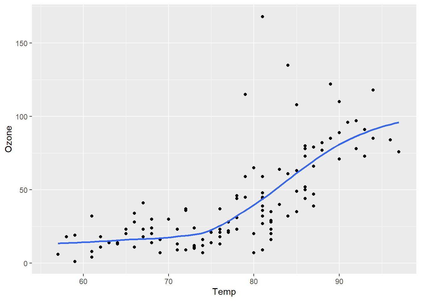
If you want to hide all of the library loading messages or kinds of output, you can customize this as well. For example to suppress warnings:
```{r}
#| warning: true

library(ggplot2)
ggplot(airquality, aes(Temp, Ozone)) +
  geom_point() +
  geom_smooth(method = "loess", se = FALSE)
```
#> `geom_smooth()` using formula = 'y ~ x'#> Warning: Removed 37 rows containing non-finite outside the scale range
#> (`stat_smooth()`).#> Warning: Removed 37 rows containing missing values or values outside the scale range
#> (`geom_point()`).
```{r}
#| warning: false

library(ggplot2)
ggplot(airquality, aes(Temp, Ozone)) +
  geom_point() +
  geom_smooth(method = "loess", se = FALSE)
```
For more options, visit https://quarto.org/docs/computations/execution-options.html