Class 15

More EDA

Materials for class on

2024-10-17

Preparation and Further Reading

R4DS chapter was assigned:

Agenda

Today we’ll focus on:

{todor} package
Homework 2 notes/questions
EDA visualization
Homework Project 1 planning

`{todor}` package and Homework 1 feedback

Working on homework and feedback gives us a chance to practice methods for collaborating on R projects - how would you share feedback or even leave better notes for yourself across time? The {todor} package with an RStudio add-in is very useful for this.

#install.packages("todor")

The package documentation explains how it is used: https://github.com/dokato/todor

Poll

What keywords can you use with todor?

This is also how you can view your feedback on your homework, if I uploaded a file on Canvas.

Homework 2 Notes

Submitting Homework 2

Since you are working with more complex projects, we are going to move towards sharing them in ways more similar to how you would share this work in collaboration outside of the classroom. You would typically share the full folder of your project, including analysis files and data (or links to the data). One way to share a full folder is by zipping it.

You can use your operating system to zip the files, or there are some functions to do this in R as well.

Cleaning up Projects

Your projects should include your analysis file (Quarto/Rmd) but also the rendered html and any other necessary data files.

To keep your project files a bit neater:

use embedded resources for your html file (avoids extra .css files, etc.)
omit the .Rproj.user folder (not needed for other users)
uncheck all of the history/environment saving options in RStudio
keep your data in a specific data folder

More Practice: `{bakeoff}` package

library(tidyverse)
library(bakeoff)

The `{bakeoff}` package

Today we’ll use the {bakeoff} package to do some new visualizations. These data are from the show “Great British Bakeoff”, known as the “Great British Baking Show” in the US. Contestants compete weekly for a whole series of episodes. Each episode has three challenges, and at the end one baker is designated “star baker” and one baker is eliminated (with some exceptions).

Let’s see what data are available:

data(package = "bakeoff")

#> Data sets in package ‘bakeoff’:
#> 
#> bakers (data)                      Bakers
#> bakers_raw (data)                  Bakers (raw)
#> bakes_raw (data)                   Bakes (raw)
#> challenges (data)                  Challenges
#> episodes (data)                    Episodes
#> episodes_raw (data)                Each episodes' challenges (raw)
#> ratings (data)                     Ratings
#> ratings_raw (data)                 Each episode's ratings (raw)
#> results_raw (data)                 Each baker's results by episode (raw)
#> seasons_raw (data)                 Data about each season aired in the US (raw)
#> series_raw (data)                  Data about each series aired in the UK (raw)
#> spice_test_wide (data)             Spice Test

Glimpse at the bakers data:

glimpse(bakers)

#> Rows: 120
#> Columns: 24
#> $ series                    <dbl> 1, 1, 1, 1, 1, 1, 1, 1, 1, 1, 2, 2, 2, 2, 2,…
#> $ baker                     <chr> "Annetha", "David", "Edd", "Jasminder", "Jon…
#> $ star_baker                <int> 0, 0, 0, 0, 0, 0, 0, 0, 0, 0, 0, 0, 0, 0, 0,…
#> $ technical_winner          <int> 0, 0, 2, 0, 1, 0, 0, 0, 2, 0, 1, 2, 0, 1, 1,…
#> $ technical_top3            <int> 1, 1, 4, 2, 1, 0, 0, 0, 4, 2, 3, 5, 1, 1, 2,…
#> $ technical_bottom          <int> 1, 3, 1, 2, 2, 1, 1, 0, 1, 2, 1, 3, 2, 6, 3,…
#> $ technical_highest         <dbl> 2, 3, 1, 2, 1, 10, 4, NA, 1, 2, 1, 1, 2, 1, …
#> $ technical_lowest          <dbl> 7, 8, 6, 5, 9, 10, 4, NA, 8, 5, 5, 6, 10, 8,…
#> $ technical_median          <dbl> 4.5, 4.5, 2.0, 3.0, 6.0, 10.0, 4.0, NA, 3.0,…
#> $ series_winner             <int> 0, 0, 1, 0, 0, 0, 0, 0, 0, 0, 0, 0, 0, 0, 0,…
#> $ series_runner_up          <int> 0, 0, 0, 0, 0, 0, 0, 0, 0, 0, 0, 0, 0, 0, 0,…
#> $ total_episodes_appeared   <dbl> 2, 4, 6, 5, 3, 1, 2, 1, 6, 6, 4, 8, 3, 7, 5,…
#> $ first_date_appeared       <date> 2010-08-17, 2010-08-17, 2010-08-17, 2010-08…
#> $ last_date_appeared        <date> 2010-08-24, 2010-09-07, 2010-09-21, 2010-09…
#> $ first_date_us             <date> NA, NA, NA, NA, NA, NA, NA, NA, NA, NA, NA,…
#> $ last_date_us              <date> NA, NA, NA, NA, NA, NA, NA, NA, NA, NA, NA,…
#> $ percent_episodes_appeared <dbl> 33.33333, 66.66667, 100.00000, 83.33333, 50.…
#> $ percent_technical_top3    <dbl> 50.00000, 25.00000, 66.66667, 40.00000, 33.3…
#> $ baker_full                <chr> "Annetha Mills", "David Chambers", "Edward \…
#> $ age                       <dbl> 30, 31, 24, 45, 25, 51, 44, 48, 37, 31, 31, …
#> $ occupation                <chr> "Midwife", "Entrepreneur", "Debt collector f…
#> $ hometown                  <chr> "Essex", "Milton Keynes", "Bradford", "Birmi…
#> $ baker_last                <chr> "Mills", "Chambers", "Kimber", "Randhawa", "…
#> $ baker_first               <chr> "Annetha", "David", "Edward", "Jasminder", "…

You can also use ?bakers for the data dictionary. And then for bakes_raw:

glimpse(bakes_raw)

#> Rows: 548
#> Columns: 6
#> $ series      <int> 1, 1, 1, 1, 1, 1, 1, 1, 1, 1, 1, 1, 1, 1, 1, 1, 1, 1, 1, 1…
#> $ episode     <int> 1, 1, 1, 1, 1, 1, 1, 1, 1, 1, 2, 2, 2, 2, 2, 2, 2, 2, 3, 3…
#> $ baker       <chr> "Annetha", "David", "Edd", "Jasminder", "Jonathan", "Lea",…
#> $ signature   <chr> "Light Jamaican Black Cakewith Strawberries and Cream", "C…
#> $ technical   <int> 2, 3, 1, NA, 9, 10, NA, NA, 8, NA, 7, 8, 6, 2, 1, 4, 3, 5,…
#> $ showstopper <chr> "Red, White & Blue Chocolate Cake with Cigarellos, Fresh F…

As needed you can do the same for the other datasets.

Poll

What variables in this dataset are categorical and nominal (unordered)?

Poll

What variables in this dataset seem ordinal (discrete but ordered)?

A bit about factors

The R type factor can be used for discrete variables that are ordered (ordinal) or unordered (nominal). Traditionally, string variables were imported as factors by default in R, but this is no longer true. If you want to make a variable a factor, you can use as.factor() or as_factor().

df_bakers <- bakers |> 
  mutate(series_fac = as.factor(series), .after = series)
df_bakers

#> # A tibble: 120 × 25
#>    series series_fac baker     star_baker technical_winner technical_top3
#>     <dbl> <fct>      <chr>          <int>            <int>          <int>
#>  1      1 1          Annetha            0                0              1
#>  2      1 1          David              0                0              1
#>  3      1 1          Edd                0                2              4
#>  4      1 1          Jasminder          0                0              2
#>  5      1 1          Jonathan           0                1              1
#>  6      1 1          Lea                0                0              0
#>  7      1 1          Louise             0                0              0
#>  8      1 1          Mark               0                0              0
#>  9      1 1          Miranda            0                2              4
#> 10      1 1          Ruth               0                0              2
#> # ℹ 110 more rows
#> # ℹ 19 more variables: technical_bottom <int>, technical_highest <dbl>,
#> #   technical_lowest <dbl>, technical_median <dbl>, series_winner <int>,
#> #   series_runner_up <int>, total_episodes_appeared <dbl>,
#> #   first_date_appeared <date>, last_date_appeared <date>,
#> #   first_date_us <date>, last_date_us <date>, percent_episodes_appeared <dbl>,
#> #   percent_technical_top3 <dbl>, baker_full <chr>, age <dbl>, …

It “looks” the same so far, except for appearing to be left-aligned in the display. But let’s look into them further.

df_bakers$series

#>   [1]  1  1  1  1  1  1  1  1  1  1  2  2  2  2  2  2  2  2  2  2  2  2  3  3  3
#>  [26]  3  3  3  3  3  3  3  3  3  4  4  4  4  4  4  4  4  4  4  4  4  4  5  5  5
#>  [51]  5  5  5  5  5  5  5  5  5  6  6  6  6  6  6  6  6  6  6  6  6  7  7  7  7
#>  [76]  7  7  7  7  7  7  7  7  8  8  8  8  8  8  8  8  8  8  8  8  9  9  9  9  9
#> [101]  9  9  9  9  9  9  9 10 10 10 10 10 10 10 10 10 10 10 10 10

df_bakers$series_fac

#>   [1] 1  1  1  1  1  1  1  1  1  1  2  2  2  2  2  2  2  2  2  2  2  2  3  3  3 
#>  [26] 3  3  3  3  3  3  3  3  3  4  4  4  4  4  4  4  4  4  4  4  4  4  5  5  5 
#>  [51] 5  5  5  5  5  5  5  5  5  6  6  6  6  6  6  6  6  6  6  6  6  7  7  7  7 
#>  [76] 7  7  7  7  7  7  7  7  8  8  8  8  8  8  8  8  8  8  8  8  9  9  9  9  9 
#> [101] 9  9  9  9  9  9  9  10 10 10 10 10 10 10 10 10 10 10 10 10
#> Levels: 1 2 3 4 5 6 7 8 9 10

Notice the new specification of “levels”. In this case they appear the same as the numbers, as the levels are set by default to be in “alphabetical” order. Let’s see what happens if we make the names into factors:

df_bakers <- df_bakers |> 
  mutate(baker_fac = as.factor(baker), .after = baker)
df_bakers$baker_fac

#>   [1] Annetha    David      Edd        Jasminder  Jonathan   Lea       
#>   [7] Louise     Mark       Miranda    Ruth       Ben        Holly     
#>  [13] Ian        Janet      Jason      Joanne     Keith      Mary-Anne 
#>  [19] Robert     Simon      Urvashi    Yasmin     Brendan    Cathryn   
#>  [25] Danny      James      John       Manisha    Natasha    Peter     
#>  [31] Ryan       Sarah-Jane Stuart     Victoria   Ali        Beca      
#>  [37] Christine  Deborah    Frances    Glenn      Howard     Kimberley 
#>  [43] Lucy       Mark       Robert     Ruby       Toby       Chetna    
#>  [49] Claire     Diana      Enwezor    Iain       Jordan     Kate      
#>  [55] Luis       Martha     Nancy      Norman     Richard    Alvin     
#>  [61] Dorret     Flora      Ian        Marie      Mat        Nadiya    
#>  [67] Paul       Sandy      Stu        Tamal      Ugnė       Andrew    
#>  [73] Benjamina  Candice    Jane       Kate       Lee        Louise    
#>  [79] Michael    Rav        Selasi     Tom        Val        Chris     
#>  [85] Flo        James      Julia      Kate       Liam       Peter     
#>  [91] Sophie     Stacey     Steven     Tom        Yan        Antony    
#>  [97] Briony     Dan        Imelda     Jon        Karen      Kim-Joy   
#> [103] Luke       Manon      Rahul      Ruby       Terry      Alice     
#> [109] Amelia     Dan        David      Helena     Henry      Jamie     
#> [115] Michael    Michelle   Phil       Priya      Rosie      Steph     
#> 107 Levels: Ali Alice Alvin Amelia Andrew Annetha Antony Beca Ben ... Yasmin

Notice that the levels are in alphabetical order. This is the way they will be sorted if we plot them:

df_bakers |> 
  filter(str_starts(baker,"D")) |> 
  ggplot(aes(x = baker_fac)) +
  geom_bar() +
  labs(title = "Count of Bakers per Name")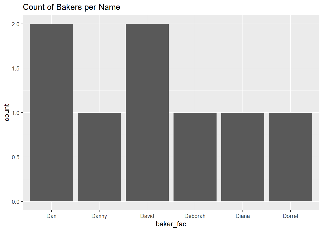

Factors also allow us to reorder, or manually set the appropriate order.

Using factor():

df_bakers <- df_bakers |> 
  mutate(series_fac2 = factor(series, 
                              levels = c("2", "4", "6", "8", "10", "1", "3", "5", "7", "9")
                              ), 
         .after = baker_fac)
df_bakers$series_fac2

#>   [1] 1  1  1  1  1  1  1  1  1  1  2  2  2  2  2  2  2  2  2  2  2  2  3  3  3 
#>  [26] 3  3  3  3  3  3  3  3  3  4  4  4  4  4  4  4  4  4  4  4  4  4  5  5  5 
#>  [51] 5  5  5  5  5  5  5  5  5  6  6  6  6  6  6  6  6  6  6  6  6  7  7  7  7 
#>  [76] 7  7  7  7  7  7  7  7  8  8  8  8  8  8  8  8  8  8  8  8  9  9  9  9  9 
#> [101] 9  9  9  9  9  9  9  10 10 10 10 10 10 10 10 10 10 10 10 10
#> Levels: 2 4 6 8 10 1 3 5 7 9

This specifies the levels with a different order than alphanumeric, which will affect how they sort, and if they are treated as ordered, can affect their statistical analysis.

Using fct_relevel():

df_bakers |> 
  filter(str_starts(baker,"D")) |> 
  ggplot(aes(x = fct_relevel(baker_fac, c("Deborah", "Dan", "Diana", "David", "Danny",  "Dorret")))) +
  geom_bar()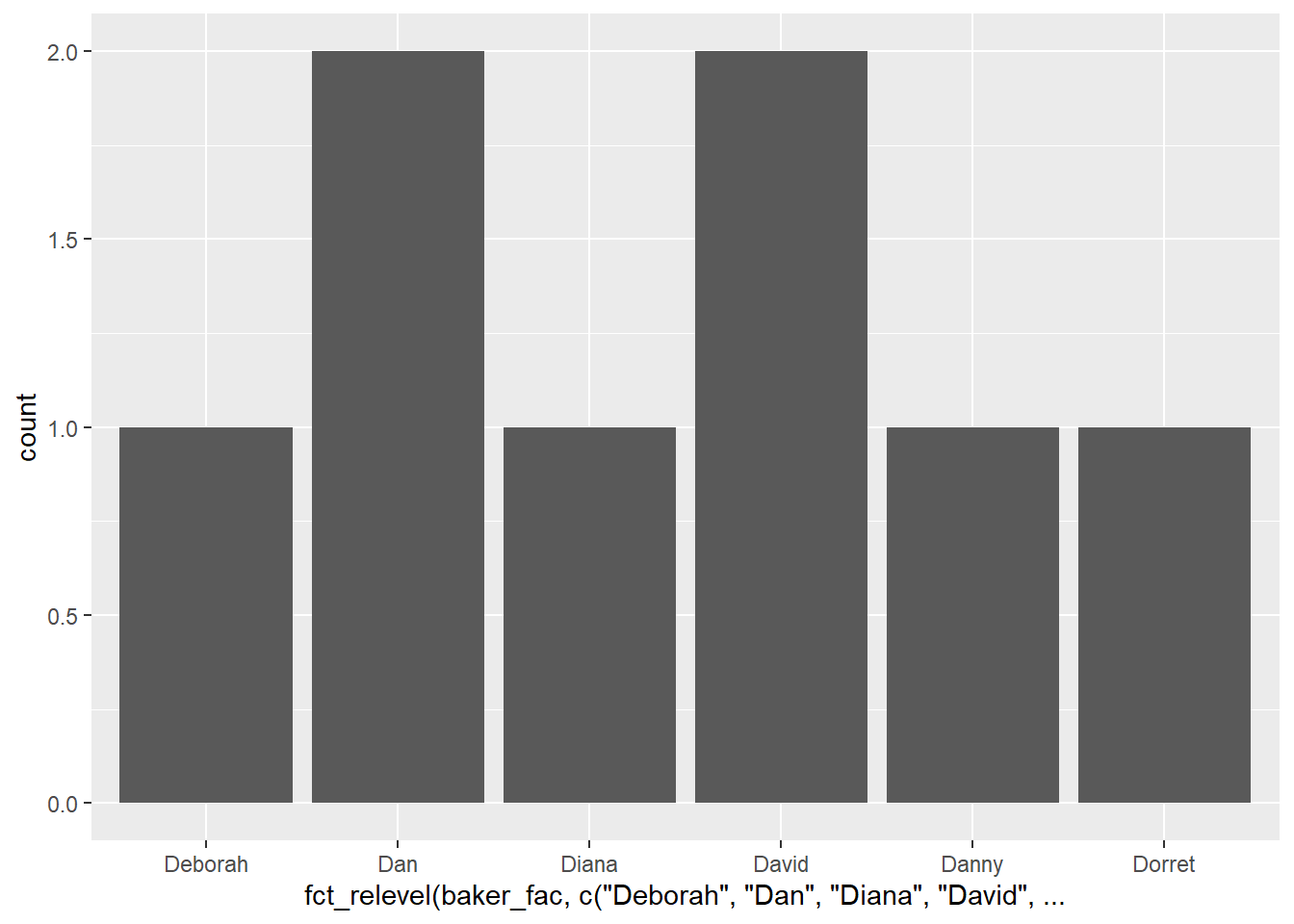

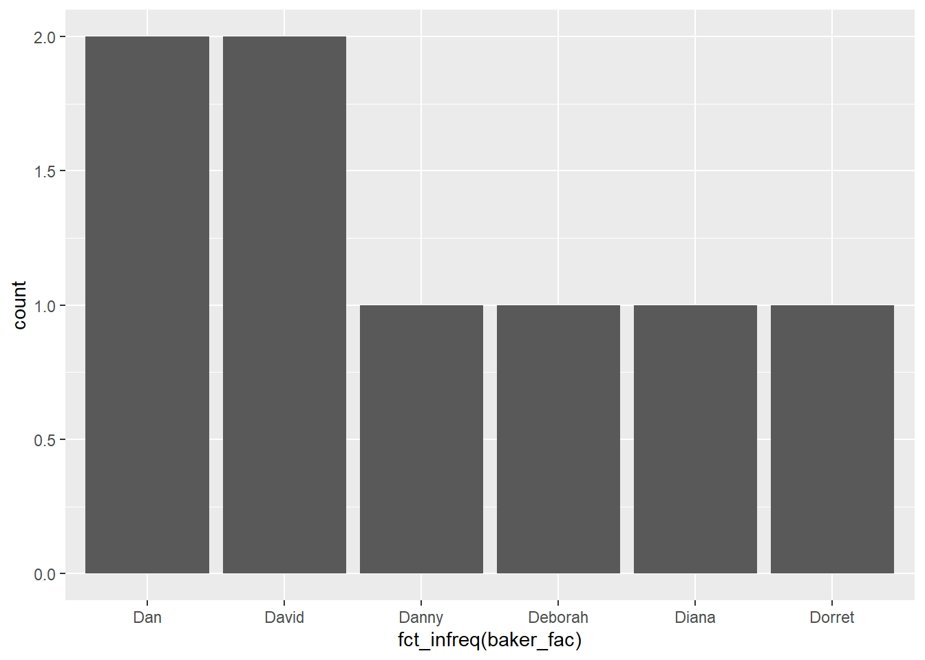
You can reorder based on the data using {forcats} functions like:

fct_inorder() - order of appearance in data
fct_infreq() - number of observations for each level, largest to smallest
fct_inseq() - numeric value of level
fct_reorder() - order by the value of another variable in the data

These can be very handy when you are plotting and want to arrange the data from big to small, for example:

df_bakers |> 
  filter(str_starts(baker,"D")) |> 
  ggplot(aes(x = fct_infreq(baker_fac))) +
  geom_bar()

You can find more about factors and level ordering in the R4DS chapter.

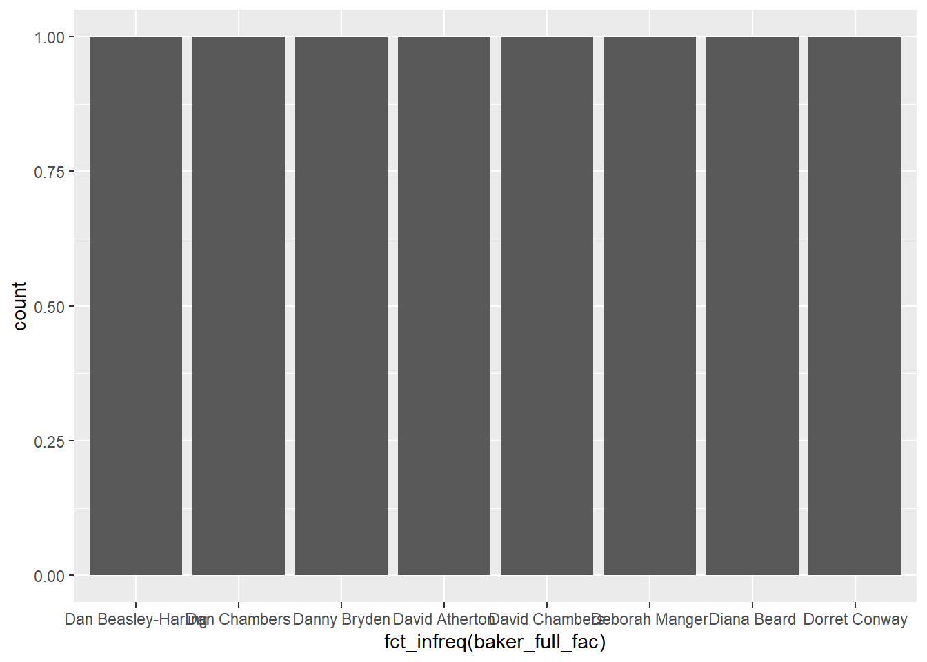
Notice that in the previous plots, we can see that there is more than one “Dan” and “David”. This is probably not a desirable represenation of the data unless we are truly analyzing something about people named “Dan”, etc. If we want to represent each baker individually, we need to make sure the variable we are using for the factors is unique. We would do this by using the full name variable:

df_bakers <- df_bakers |> 
  mutate(baker_full_fac = as.factor(baker_full), .after = baker_full)
df_bakers$baker_full_fac

#>   [1] Annetha Mills           David Chambers          Edward "Edd" Kimber    
#>   [4] Jasminder Randhawa      Jonathan Shepherd       Lea Harris             
#>   [7] Louise Brimelow         Mark Whithers           Miranda Gore Browne    
#>  [10] Ruth Clemens            Ben Frazer              Holly Bell             
#>  [13] Ian Vallance            Janet Basu              Jason White            
#>  [16] Joanne "Jo" Wheatley    Keith Batsford          Mary-Anne Boermans     
#>  [19] Robert Billington       Simon Blackwell         Urvashi Roe            
#>  [22] Yasmin Limbert          Brendan Lynch           Cathryn Dresser        
#>  [25] Danny Bryden            James Morton            John Whaite            
#>  [28] Manisha Parmar          Natasha Stringer        Peter Maloney          
#>  [31] Ryan Chong              Sarah-Jane Willis       Stuart Marston-Smith   
#>  [34] Victoria Chester        Ali Imdad               Beca Lyne-Pirkis       
#>  [37] Christine Wallace       Deborah Manger          Frances Quinn          
#>  [40] Glenn Cosby             Howard Middleton        Kimberley Wilson       
#>  [43] Lucy Bellamy            Mark Onley              Robert Smart           
#>  [46] Ruby Tandoh             Toby Waterworth         Chetna Makan           
#>  [49] Claire Goodwin          Diana Beard             Enwezor Nzegwu         
#>  [52] Iain Watters            Jordan Cox              Kate Henry             
#>  [55] Luis Troyano            Martha Collison         Nancy Birtwhistle      
#>  [58] Norman Calder           Richard Burr            Alvin Magallanes       
#>  [61] Dorret Conway           Flora Shedden           Ian Cumming            
#>  [64] Marie Campbell          Mat Riley               Nadiya Hussain         
#>  [67] Paul Jagger             Sandy Docherty          Stu Henshall           
#>  [70] Tamal Ray               Ugnė Bubnaityte         Andrew Smyth           
#>  [73] Benjamina Ebuehi        Candice Brown           Jane Beedle            
#>  [76] Kate Barmby             Lee Banfield            Louise Williams        
#>  [79] Michael Georgiou        Rav Bansal              Selasi Gbormittah      
#>  [82] Tom Gilliford           Valerie "Val" Stones    Chris Geiger           
#>  [85] Flo Atkins              James Hillery           Julia Chernogorova     
#>  [88] Kate Lyon               Liam Charles            Peter Abatan           
#>  [91] Sophie Faldo            Stacey Hart             Steven Carter-Bailey   
#>  [94] Tom Hetherington        Chuen-Yan "Yan" Tsou    Antony Amourdoux       
#>  [97] Briony Williams         Dan Beasley-Harling     Imelda McCarron        
#> [100] Jon Jenkins             Karen Wright            Kim-Joy Hewlett        
#> [103] Luke Thompson           Manon Lagrève           Rahul Mandal           
#> [106] Ruby Bhogal             Terry Hartill           Alice Fevronia         
#> [109] Amelia Le Bruin         Dan Chambers            David Atherton         
#> [112] Helena Garcia           Henry Bird              Jamie Finn             
#> [115] Michael Chakraverty     Michelle Evans-Fecci    Phil Thorne            
#> [118] Priya O'Shea            Rosie Brandreth-Poynter Steph Blackwell        
#> 120 Levels: Ali Imdad Alice Fevronia Alvin Magallanes ... Yasmin Limbert

Now there are 120 levels, which matches the number of rows in the dataset.

df_bakers |> 
  filter(str_starts(baker,"D")) |> 
  ggplot(aes(x = fct_infreq(baker_full_fac))) +
  geom_bar()

Visualizing Relationships

Remember when we’re exploring data, we want to consider the variables that we want to consider “together”. Let’s try out some new examples.

Viewers by Episode

Poll

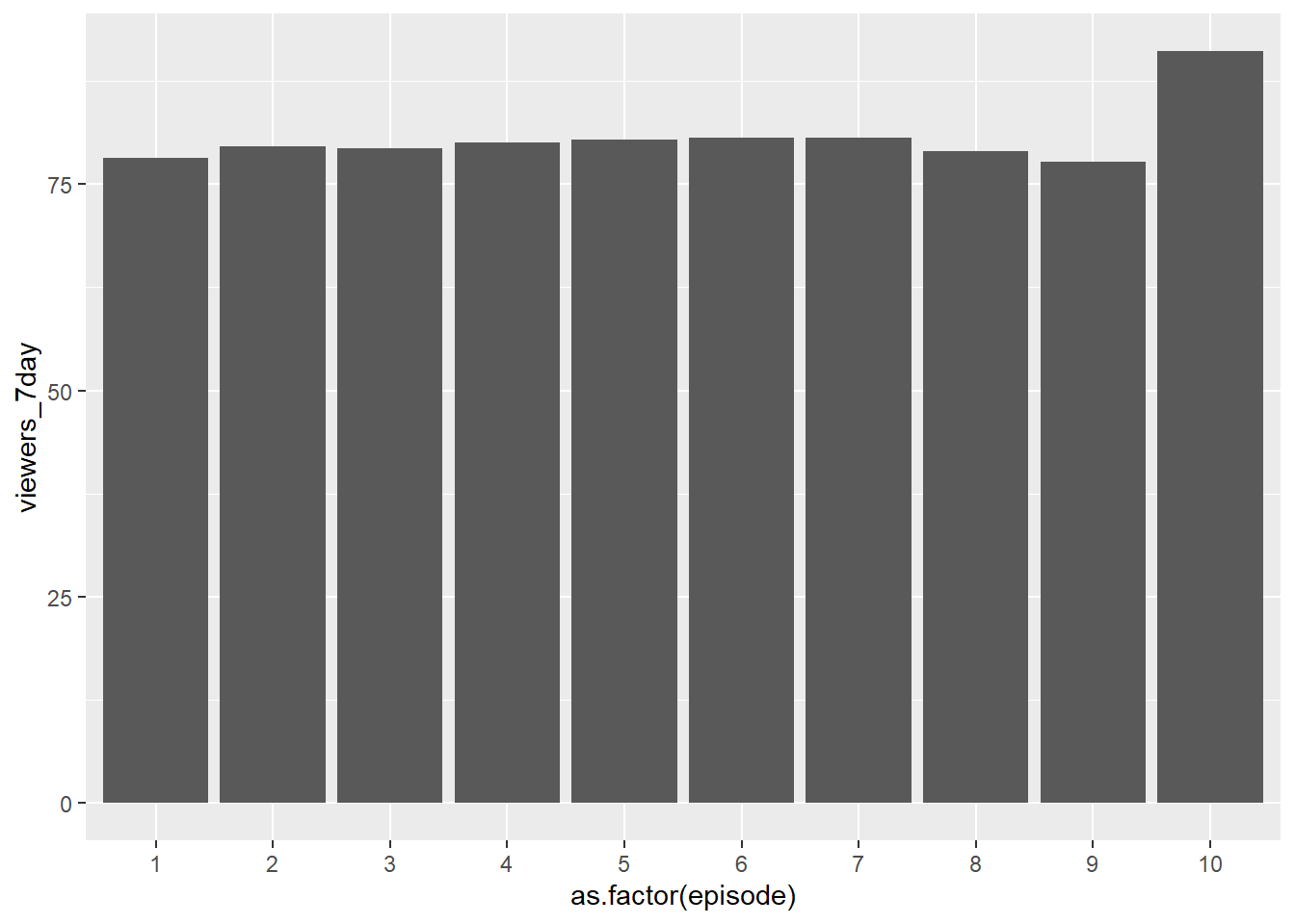
Is there a relationship between episode number and number of viewers?

Episode number is categorical and number of viewers is continuous. We could use a column plot to show the total viewers across all series:

ggplot(ratings, aes(x = as.factor(episode), y = viewers_7day))+
  geom_col()

Here’s another example using summarize() to calculate the sum of viewers before piping into ggplot():

ratings |> 
  group_by(episode) |>
  summarize(total_viewers_7day = sum(viewers_7day)) |> 
  ggplot(aes(x= as.factor(episode), y = total_viewers_7day, group = 1))+
  geom_line()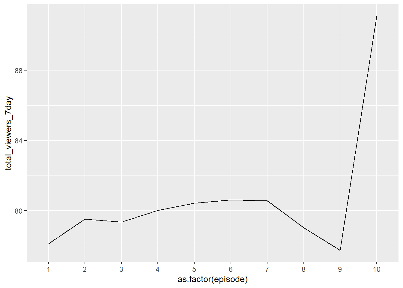

In this case, group = 1 sets a kind of default grouping for the line. This is necessary when there is a factor on the x axis, as the true default doesn’t work in this case. You would get a plot without a line and a warning like this:

ratings |> 
  group_by(episode) |>
  summarize(total_viewers_7day = sum(viewers_7day)) |> 
  ggplot(aes(x= as.factor(episode), y = total_viewers_7day)) +
  geom_line()

#> `geom_line()`: Each group consists of only one observation.
#> ℹ Do you need to adjust the group aesthetic?

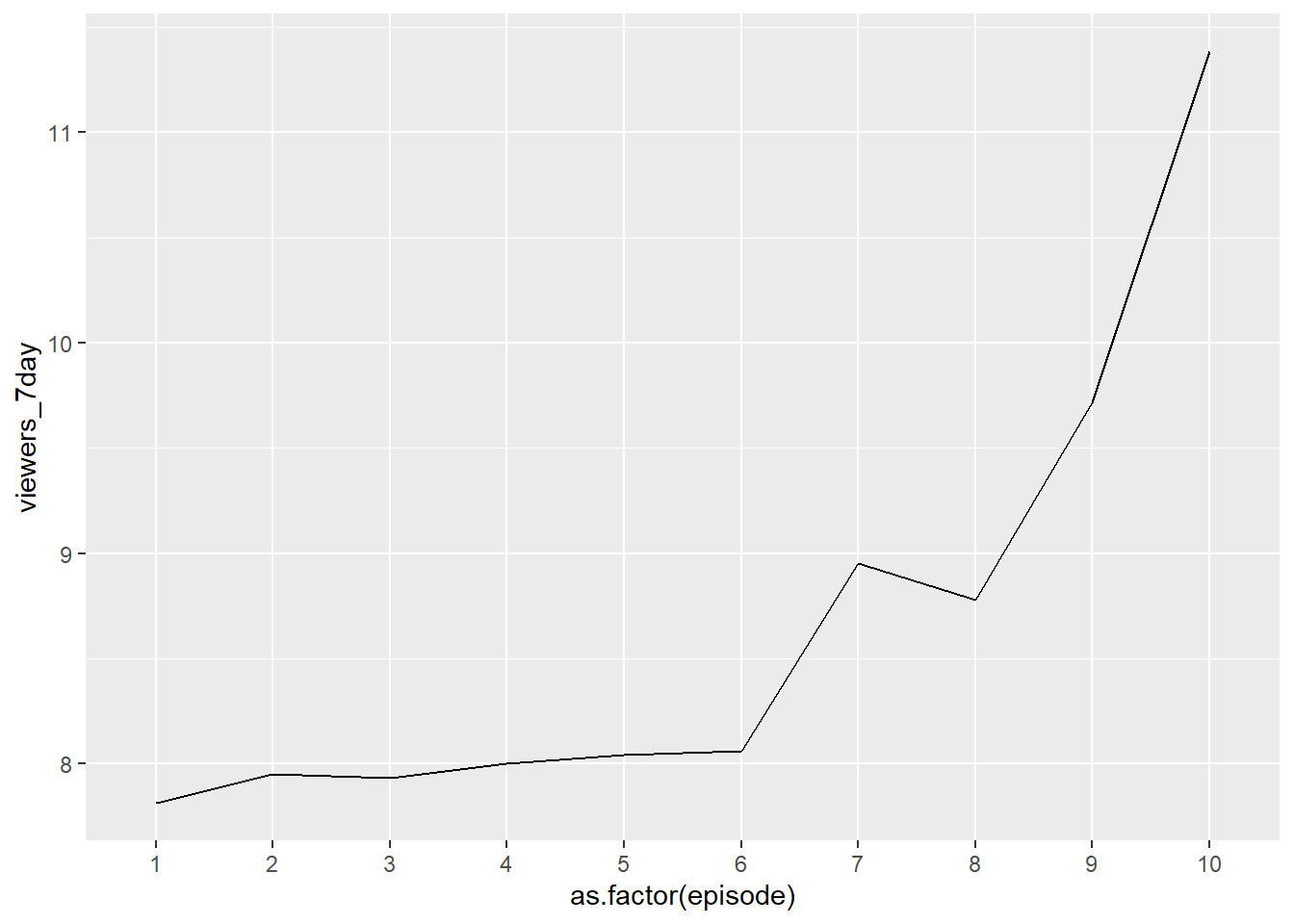
We could also use ggplot() to summarize, and maybe use mean instead of the sum (depending on what we are trying to see):

ratings |> 
  ggplot(aes(x= as.factor(episode), y = viewers_7day, group = 1))+
  geom_line(stat = "summary", fun = "mean")

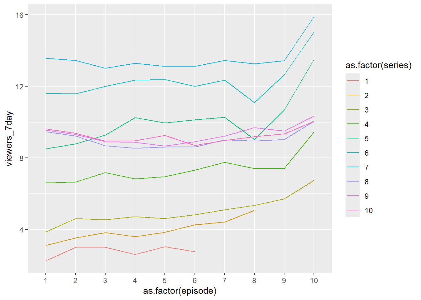
Viewers by Episode by Series

Poll

What if we want to see the pattern for each series? Add the variable of series to the plot.

Here we don’t need to summarize as we are plotting the numbers in the dataset directly. We can use as.factor() to treat episode and series as factors, or we could have made these factors in the underlying dataframe if that is what we want for other uses of the data.

ggplot(ratings, aes(x= as.factor(episode), y = viewers_7day, 
                    group = as.factor(series),
                    color = as.factor(series)))+
  geom_line()

Age and Number of Episodes

Total number of episodes is a measure of how far bakers made it into the series (that is, how successful they were). Is there a correlation between age and success?

ggplot(bakers, aes(x = age, y = total_episodes_appeared)) +
  geom_point() +
  geom_smooth(method = lm) +
  scale_y_continuous(breaks = 1:10)

#> `geom_smooth()` using formula = 'y ~ x'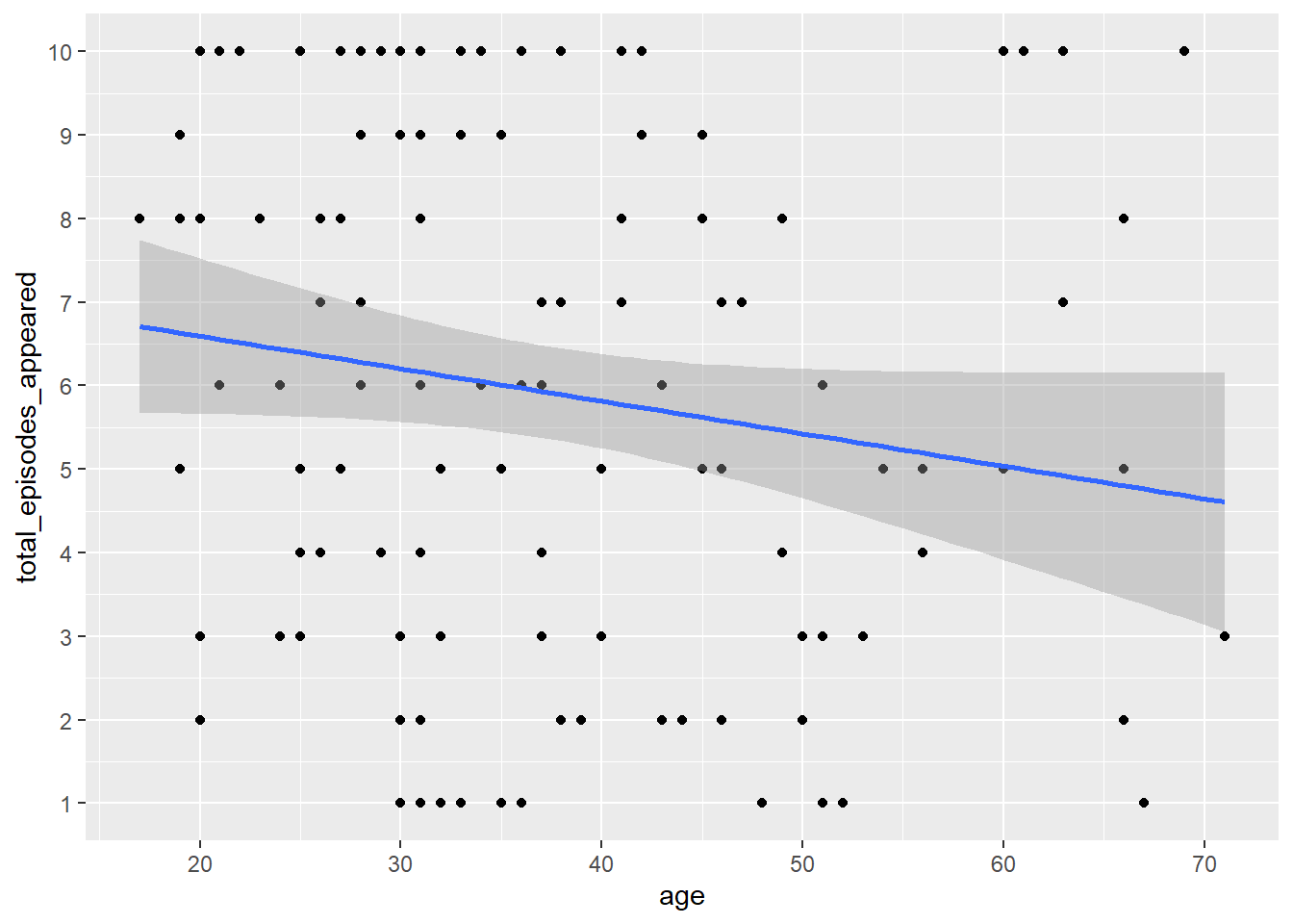

Note there are not as many participants above 60, so we could look just at those 60 and under. xlim() will remove data outside of the specified limits, so the slope of the line will change:

ggplot(bakers, aes(x = age, y = total_episodes_appeared)) +
  geom_point() +
  geom_smooth(method = lm) +
  scale_y_continuous(breaks = 1:10) +
  xlim(15, 60)

#> `geom_smooth()` using formula = 'y ~ x'

#> Warning: Removed 10 rows containing non-finite outside the scale range
#> (`stat_smooth()`).

#> Warning: Removed 10 rows containing missing values or values outside the scale range
#> (`geom_point()`).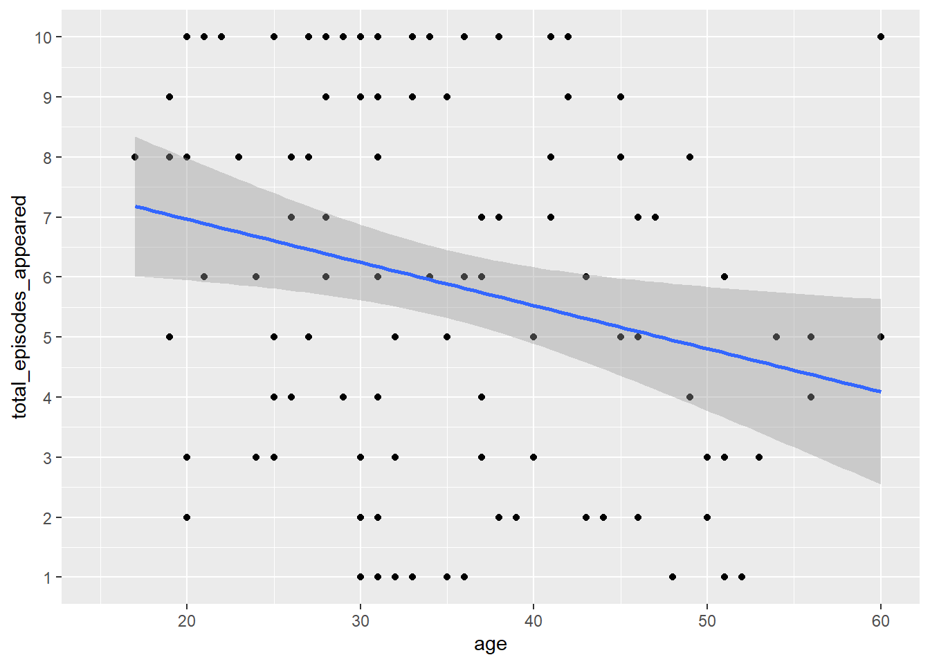

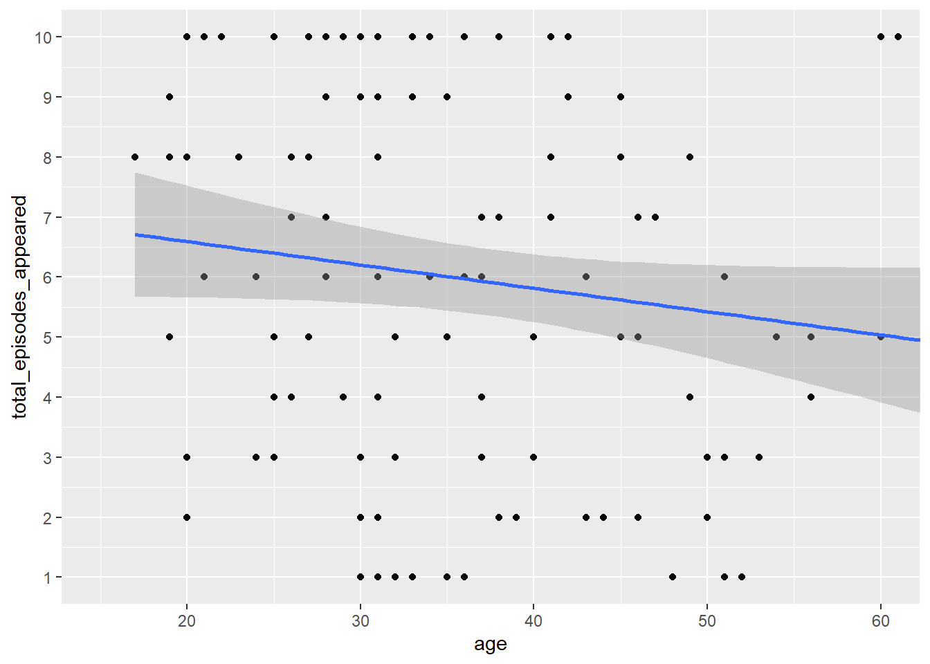
To make the plot smaller without removing underlying data, use coord_cartesian():

ggplot(bakers, aes(x = age, y = total_episodes_appeared)) +
  geom_point() +
  geom_smooth(method = lm) +
  scale_y_continuous(breaks = 1:10) +
  coord_cartesian(xlim = c(15,60))

#> `geom_smooth()` using formula = 'y ~ x'

Technical Score and Number of Episodes

How does median technical rank across episodes for each baker correlate with total number of episodes?

ggplot(bakers, aes(x = total_episodes_appeared, y = technical_median)) +
  geom_point() +
  geom_smooth(method = lm) +
  scale_y_continuous(breaks = 1:13) +
  scale_x_continuous(breaks = 1:10)

#> `geom_smooth()` using formula = 'y ~ x'

#> Warning: Removed 1 row containing non-finite outside the scale range
#> (`stat_smooth()`).

#> Warning: Removed 1 row containing missing values or values outside the scale range
#> (`geom_point()`).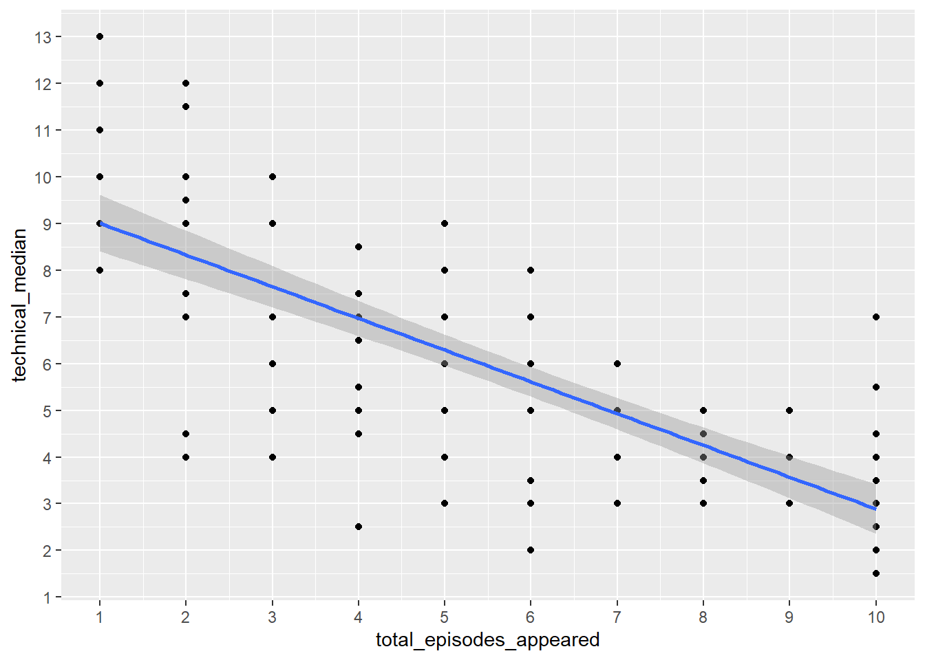

Fixing up Plots

When you’re happy with your plot choice and variables, you can turn to fixing and refining other aspects of the visualization.

Consider the following:

titles
labels
grouping of labels
axis labels and breaks
use of color, shape, linetype, etc.
relative sizing
accessibility
fonts

Axis Breaks

The breaks that show on your axes will be influenced by the underlying data and can be adjusted by modifying the data or modifying the way it is labeled and scaled to the axis.

You may want, for example, to make sure that a number is treated as a discrete factor, rather than a continuous numeric, so that non-integer breaks aren’t used, using as.factor().

You can also set breaks using scale functions, such as scale_x_discrete(breaks = c(2,4,6,8)).

Preparation and Further Reading

Agenda

{todor} package and Homework 1 feedback

Homework 2 Notes

Submitting Homework 2

Cleaning up Projects

More Practice: {bakeoff} package

The {bakeoff} package

A bit about factors

Visualizing Relationships

Viewers by Episode

Viewers by Episode by Series

Age and Number of Episodes

Technical Score and Number of Episodes

Fixing up Plots

Axis Breaks

`{todor}` package and Homework 1 feedback

More Practice: `{bakeoff}` package

The `{bakeoff}` package