Class 25

Cool Stuff

Materials for class on

2024-11-21

Agenda

Today we’ll focus on:

Cool Stuff to Know About (maybe for hp2)
Rendering Quarto to different outputs
Homework 4 Questions (10 minutes)

Cool Stuff (for Linguistics)

This is a sampling of cool things you can do for linguistics in R that we haven’t even gotten to discuss. They all interact with/depend on the basic data wrangling and analysis tools we have been learning though!

`udpipe` for Universal Dependencies Tools

https://bnosac.github.io/udpipe/en/

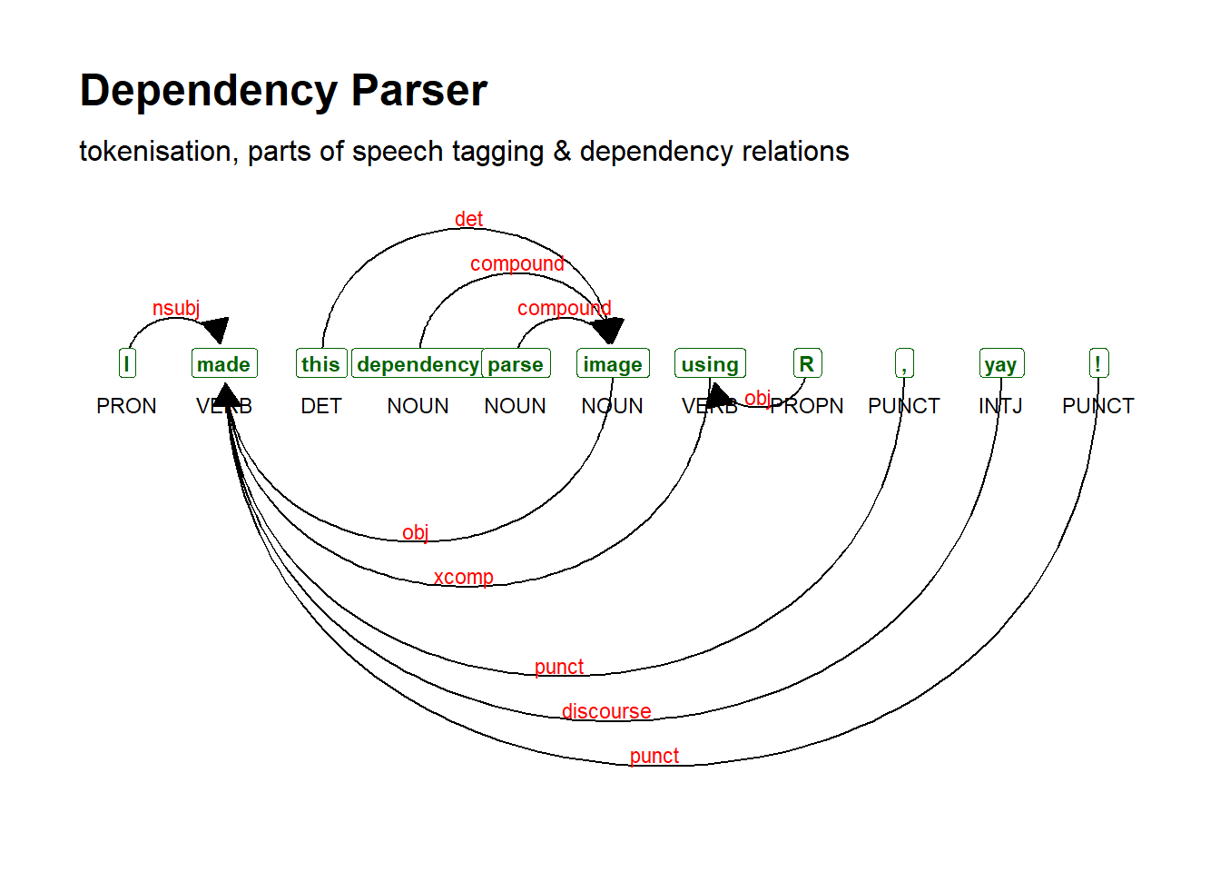
{udpipe} provides some very cool language analysis tools. Possibly the most useful function we haven’t talked about in class is Part of Speech tagging, and it also creates dependency parses, which are a representation of intra-sentence relationships that are different from the constituency parses you may be more familiar with. These are based on the Universal Dependencies resource, which has the benefit of coverage for over 100 languages. Constituency- based treebanks are not as widely available.

#install.packages(udpipe)
#install.packages(textplot)
#install.packages(ggraph)
library(udpipe)
library(textplot)

We choose and download the model we want to use:

udmodel <- udpipe_download_model(language = "english")
udmodel <- udpipe_load_model(file = udmodel$file_model)

Then annotate our text:

y <- udpipe(x = "I made this dependency parse image using R, yay!", object = "english") 
y |> select(-sentence) |> kbl() |> kable_styling()

doc_id	paragraph_id	sentence_id	start	end	term_id	token_id	token	lemma	upos	xpos	feats	head_token_id	dep_rel	deps	misc
doc1	1	1	1	1	1	1	I	I	PRON	PRP	Case=Nom\|Number=Sing\|Person=1\|PronType=Prs	2	nsubj	NA	NA
doc1	1	1	3	6	2	2	made	make	VERB	VBD	Mood=Ind\|Tense=Past\|VerbForm=Fin	0	root	NA	NA
doc1	1	1	8	11	3	3	this	this	DET	DT	Number=Sing\|PronType=Dem	6	det	NA	NA
doc1	1	1	13	22	4	4	dependency	dependency	NOUN	NN	Number=Sing	6	compound	NA	NA
doc1	1	1	24	28	5	5	parse	parse	NOUN	NN	Number=Sing	6	compound	NA	NA
doc1	1	1	30	34	6	6	image	image	NOUN	NN	Number=Sing	2	obj	NA	NA
doc1	1	1	36	40	7	7	using	use	VERB	VBG	VerbForm=Ger	2	xcomp	NA	NA
doc1	1	1	42	42	8	8	R	R	PROPN	NNP	Number=Sing	7	obj	NA	SpaceAfter=No
doc1	1	1	43	43	9	9	,	,	PUNCT	,	NA	2	punct	NA	NA
doc1	1	1	45	47	10	10	yay	yay	INTJ	UH	NA	2	discourse	NA	SpaceAfter=No
doc1	1	1	48	48	11	11	!	!	PUNCT	.	NA	2	punct	NA	SpacesAfter=\n

Use the dependency plotter from {textplot}:

textplot_dependencyparser(y)

#> Loading required namespace: ggraph

The same author has created several other related packages: https://bnosac.github.io/udpipe/docs/doc9.html

`quanteda` for Text Analysis

https://quanteda.io/

{quanteda} is one of the most well-known text analysis packages for R. It actually is a family of packages that can be used for NLP, text management, modelling, statistics, and plotting.

`readtext` (quanteda)

https://readtext.quanteda.io/index.html

The {readtext} package can import text from all sorts of files, including PDFs. See the reference for examples of how to read in a whole folder of PDF files and extract the text! It can do the same for CSV, txt, Microsoft Word, JSON, etc.

Language Variation and Change Analysis in R

Tutorial by Matt Hunt Gardner:

https://lingmethodshub.github.io/content/R/lvc_r/010_lvcr.html

`lingtypology` package

https://github.com/ropensci/lingtypology

{lingtypology} provides tools for searching typology and cartography databases and working with that data.

Praat Helpers

The University of Minnesota ListenLab has gathered some Praat helper scripts: https://github.com/ListenLab/Praat

There are some other R tools for speech in other repos of theirs as well.

Phylogenetic Trees

A tutorial on creating phylogenetic trees by Erich Round:

https://ladal.edu.au/phylo

Working with Maps

Josef Fruehwald has some great teaching materials, and has some guidance for starting on maps here:

https://jofrhwld.github.io/AandS500_2023/class_notes/2023-02-28/

A JSON API data Tutorial

From Thomas Mock:

https://themockup.blog/posts/2020-12-13-extracting-json-from-websites-and-public-apis-with-r/

`plotly`

{plotly} is a plotting package that can be used with or without ggplot, based on the JavaScript library plotly.js.

https://plotly.com/r/

It gives tools for interactivity and for other types of plots such as 3D.

Here’s an example of the interactivity:

library(plotly)

g <- ggplot(faithful, aes(x = eruptions, y = waiting)) +
  stat_density_2d(aes(fill = after_stat(level)), geom = "polygon") + 
  xlim(1, 6) + ylim(40, 100)
ggplotly(g)

Here’s a 3D plot:

plot_ly(z = ~volcano, type = "surface")

`shiny` for interactive sites/apps

For the real interactive power and web-based apps, you want {shiny}. It is its own universe!

https://shiny.rstudio.com/

Packages with Python Connections

Using Python from R with `reticulate`

https://github.com/rstudio/reticulate

You may sometimes want to use Python tools/packages for a portion of your analysis, but still do the bulk of your analysis and visualization in R. Each has its strengths, and combining them is very handy!

The {reticulate} package allows you to run Python from within R. Quarto also permits this in slightly more streamlined fashion. Either way, you do need to have Python installed and deal with relevant Python environment management issues that we can’t get into in this class.

`pangoling` for word probabilities (in development)

The {pangoling} package by Bruno Nicenboim is in early development, but provides some easy tools to directly extract word probabilities from language models on HuggingFace, which is something that psycholinguists are often interested in doing.

https://bruno.nicenboim.me/pangoling/

It is not on CRAN, so you would need to install from GitHub using {remotes}.

spacyR

You can use the Python spacy package within R using {reticulate} more easily through the {spacyr} package:

https://cran.r-project.org/web/packages/spacyr/vignettes/using_spacyr.html

Transformers with R

The {text} package helps with using transformer language models from HuggingFace for NLP/ML. The package provides guidance for installing the Python packages needed to use it.

You could use this package for text generation, extracting word probabilities and embeddings, training word embeddings, computing semantic distances, and other tasks like classification.

For background on word embeddings, here’s a guide (conceptual, not R specific): https://jalammar.github.io/illustrated-word2vec/

This package is quite comprehensive, so takes a while to learn all of the capabilities.

https://r-text.org//index.html

Rendering Quarto to Other Outputs

Poll

Have you ever used LaTeX for typesetting?

Inline R Code Reminder

You can use what is called “inline R code” in Rmarkdown and Quarto documents to include variables from the environment directly in your markdown text. For example, let’s look at the msleep dataset:

library(tidyverse)
msleep

#> # A tibble: 83 × 11
#>    name   genus vore  order conservation sleep_total sleep_rem sleep_cycle awake
#>    <chr>  <chr> <chr> <chr> <chr>              <dbl>     <dbl>       <dbl> <dbl>
#>  1 Cheet… Acin… carni Carn… lc                  12.1      NA        NA      11.9
#>  2 Owl m… Aotus omni  Prim… <NA>                17         1.8      NA       7  
#>  3 Mount… Aplo… herbi Rode… nt                  14.4       2.4      NA       9.6
#>  4 Great… Blar… omni  Sori… lc                  14.9       2.3       0.133   9.1
#>  5 Cow    Bos   herbi Arti… domesticated         4         0.7       0.667  20  
#>  6 Three… Brad… herbi Pilo… <NA>                14.4       2.2       0.767   9.6
#>  7 North… Call… carni Carn… vu                   8.7       1.4       0.383  15.3
#>  8 Vespe… Calo… <NA>  Rode… <NA>                 7        NA        NA      17  
#>  9 Dog    Canis carni Carn… domesticated        10.1       2.9       0.333  13.9
#> 10 Roe d… Capr… herbi Arti… lc                   3        NA        NA      21  
#> # ℹ 73 more rows
#> # ℹ 2 more variables: brainwt <dbl>, bodywt <dbl>

I can use inline R code to tell you in the text that there are 83 rows in the dataset. What I really wrote there (you can check in the page code!) is in backticks with an r at the beginning like `r `.

I can also use this for computations, so I could calculate the mean of body weights in the dataframe, which comes out to 166.1363494.

And, I could use it to “print” statistical test output, like coefficient estimates and p-values. This is how you do simple linear models in R, by the way!

model <- lm(brainwt ~ bodywt, data = msleep)
summary(model)

#> 
#> Call:
#> lm(formula = brainwt ~ bodywt, data = msleep)
#> 
#> Residuals:
#>      Min       1Q   Median       3Q      Max 
#> -0.78804 -0.08422 -0.07634 -0.02839  2.06190 
#> 
#> Coefficients:
#>              Estimate Std. Error t value Pr(>|t|)    
#> (Intercept) 8.592e-02  4.821e-02   1.782   0.0804 .  
#> bodywt      9.639e-04  5.027e-05  19.176   <2e-16 ***
#> ---
#> Signif. codes:  0 '***' 0.001 '**' 0.01 '*' 0.05 '.' 0.1 ' ' 1
#> 
#> Residual standard error: 0.3526 on 54 degrees of freedom
#>   (27 observations deleted due to missingness)
#> Multiple R-squared:  0.8719, Adjusted R-squared:  0.8696 
#> F-statistic: 367.7 on 1 and 54 DF,  p-value: < 2.2e-16

The estimate of the impact of body weight on brain weight is 0.00096 and the associated p-value is 9.2e-26. (One would ideally format these numbers better, which there are ways to do, but not today’s topic! Quick example is using format.pval() for the p-value to get <0.001.)

These statistics are associated with the line you see in this plot (though I trimmed the scales/data using coord_cartesian() so you can see it better):

ggplot(msleep, aes(x = bodywt, y = brainwt))+
  geom_point()+
  geom_smooth(method = "lm") +
  coord_cartesian(xlim = c(0,600), ylim = c(0,2))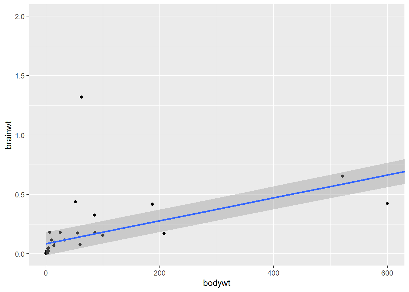

You can see the Quarto documentation about this for more details/examples.

Other Quarto Output

We’ve been focusing on making webpages/html with Quarto, but the beauty of Quarto and markdown is that it can make all different kinds of output from the same or similar documents!

The main difference is in setting your YAML format, and rendering to that specific format. However there are some quirks to customize for output, especially for PDFs based on LaTeX and slides.

For example, to render a PDF (using LaTeX), your YAML would minimally look like:

---
title: "This is going to be a PDF!"
format: pdf
---

You can specify multiple formats, with options (or default) for each:

---
title: "This is going to be a PDF!"
format: 
  html:
    embed-resources: true
  docx: default
  gfm: default
  pdf: 
    documentclass: article
    cite-method: natbib
    indent: false
    papersize: letter
---

Try it out on a document yourself (start with only one option at a time). To use LaTeX for creating PDFs, you will need to install a TeX distribution. The simplest way to do this is using the Quarto command line in your terminal (not console) to install tinytex:

Terminal

quarto install tinytex

Then create a template Quarto document, specify pdf format, and try to render!

Poll

Did it work to create a PDF?

We’ll look at some examples with various output, but here is the documentation for the different formats to follow up with:

LaTeX PDF
Typst PDF
MS Word
GitHub Markdown - good for viewable pages on GitHub, like the readme.md
Revealjs (Web) Slides
PowerPoint Slides

Agenda

Cool Stuff (for Linguistics)

udpipe for Universal Dependencies Tools

quanteda for Text Analysis

readtext (quanteda)

Language Variation and Change Analysis in R

lingtypology package

Praat Helpers

Phylogenetic Trees

Working with Sociophonetic Data in R

Plotting Vowels in R

Various Case Studies from LADAL

Working with Maps

A JSON API data Tutorial

plotly

shiny for interactive sites/apps

Packages with Python Connections

Using Python from R with reticulate

pangoling for word probabilities (in development)

spacyR

Transformers with R

Rendering Quarto to Other Outputs

Inline R Code Reminder

Other Quarto Output

`udpipe` for Universal Dependencies Tools

`quanteda` for Text Analysis

`readtext` (quanteda)

`lingtypology` package

`plotly`

`shiny` for interactive sites/apps

Using Python from R with `reticulate`

`pangoling` for word probabilities (in development)