Class 26
Collecting Data, and a Smidgen of Statistics and ML
Agenda
Today we’ll focus on:
- the importance of data visualization
- data collection tools and pointers
- Just enough statistics to be dangerous
- a hint towards ML strategies
The Importance of Data Visualization
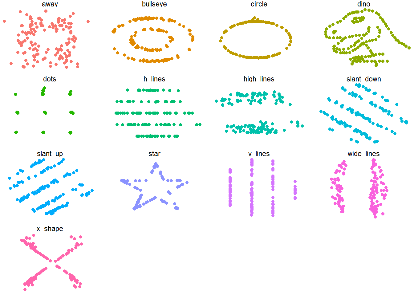
You might think from reading research articles that statistics is all that really matters, and visualization is just for fun human engagement. It’s not just a pretty way to look at summary or even inferential statistics though! Data visualization shows things that do not “appear” in summaries. The most famous illustration of this is Anscombe’s Quartet, which you can explore with the {anscombe} package. There’s a more amusing version that has garnered attention, through Alberto Cairo’s tweeted “datasaurus”. This concept is now realized in the {datasauRus} package.
You can see that the summary statistics for the multiple datasets are nearly identical:
datasaurus_dozen  |>
    group_by(dataset) |>
    summarize(
      mean_x    = mean(x),
      mean_y    = mean(y),
      std_dev_x = sd(x),
      std_dev_y = sd(y),
      corr_x_y  = cor(x, y)
    )
#> # A tibble: 13 × 6
#> dataset mean_x mean_y std_dev_x std_dev_y corr_x_y
#> <chr> <dbl> <dbl> <dbl> <dbl> <dbl>
#> 1 away 54.3 47.8 16.8 26.9 -0.0641
#> 2 bullseye 54.3 47.8 16.8 26.9 -0.0686
#> 3 circle 54.3 47.8 16.8 26.9 -0.0683
#> 4 dino 54.3 47.8 16.8 26.9 -0.0645
#> 5 dots 54.3 47.8 16.8 26.9 -0.0603
#> 6 h_lines 54.3 47.8 16.8 26.9 -0.0617
#> 7 high_lines 54.3 47.8 16.8 26.9 -0.0685
#> 8 slant_down 54.3 47.8 16.8 26.9 -0.0690
#> 9 slant_up 54.3 47.8 16.8 26.9 -0.0686
#> 10 star 54.3 47.8 16.8 26.9 -0.0630
#> 11 v_lines 54.3 47.8 16.8 26.9 -0.0694
#> 12 wide_lines 54.3 47.8 16.8 26.9 -0.0666
#> 13 x_shape 54.3 47.8 16.8 26.9 -0.0656However the underlying data are very different!
Why Inferential Statistics?
Let’s look at the data from the Husband 2022 paper.
df_all <- read.csv(here("classes", "_data", "delong maze 40Ss.csv"),
  header = 1, sep = ",", comment.char = "#", strip.white = T,
  col.names = c("Index", "Time", "Counter", "Hash", "Owner",
                "Controller", "Item", "Element", "Type", "Group",
                "FieldName", "Value", "WordNum", "Word", "Alt",
                "WordOn", "CorrWord", "RT", "Sent", "TotalTime",
                "Question", "Resp", "Acc", "RespRT")
)
Here I’ll just give you an example of translating some of the code from the original analysis into tidyverse style:
df_rt <- df_all |>
  filter(Controller == "Maze" & !str_detect(Type, "prac")) |>
  select(1:10, 13:20) |>
  separate(col = Type,
           into = c("exp", "item", "expect", "position", "pos",
                    "cloze", "art.cloze", "n.cloze"),
           sep = "\\.", convert = TRUE, fill = "right") |>
  mutate(WordNum = as.numeric(WordNum),
         Acc = as.numeric(as.character(recode(CorrWord, yes = "1", no = "0"))),
         n.cloze.scale =  scale(n.cloze),
         art.cloze.scale = scale(art.cloze)) |>
  mutate(across(where(is.character), as.factor)) |>
  filter(item != 29) |>
  filter(Hash != "9dAvrH0+R6a0U5adPzZSyA")
rt.s.filt <- df_rt |>
mutate(rgn.fix = WordNum - pos + 1,
word.num.z = scale(WordNum),
word.len = nchar(as.character(Word)),
Altword.len = nchar(as.character(Alt)),
expect = `contrasts<-`(expect,TRUE, c(-.5,.5)),
item.expect = paste(item, expect, sep=".")
) |>
filter(!Hash %in% c("gyxidIf0fqXBM7nxg2K7SQ","f8dC3CkleTBP9lUufzUOyQ"))
rgn.rt.raw <- rt.s.filt %>%
filter(rgn.fix > -4 & rgn.fix < 5) %>%
filter(Acc == 1) %>%
group_by(rgn.fix, expect) %>%
summarize(n = n(), subj = length(unique(Hash)), rt = mean(RT),
sd = sd(RT), stderr = sd / sqrt(subj)) %>%
as.data.frame()
rgn.rt.raw$rgn <- as.factor(recode(rgn.rt.raw$rgn.fix, "-3"="CW-3", "-2"="CW-2", "-1"="CW-1", "0"="art", "1"="n","2"="CW+1", "3"="CW+2", "4"="CW+3"))
rgn.rt.raw$rgn <- ordered(rgn.rt.raw$rgn, levels = c("CW-3", "CW-2", "CW-1", "art", "n", "CW+1", "CW+2", "CW+3"))Zooming in on the article responses, and looking at the grand averaged data :
rt.s.filt |>
  filter(rgn.fix == 0) |>
  group_by(Hash, expect) |>
  summarize(RT = mean(RT, na.rm = TRUE)) |>
  group_by(expect) |>
  summarize(RT = mean(RT, na.rm = TRUE)) |>
  gt() |>
fmt_number(decimals = 0)| expect | RT |
|---|---|
| expected | 672 |
| unexpected | 717 |
The unexpected articles took longer than the expected ones, judging by the mean. But it’s only by 45 milliseconds. How much variance is there underneath that mean? Look at the individual points, representing participants.
set.seed(343)
p_parts <- rt.s.filt |>
  filter(rgn.fix == 0) |>
  group_by(Hash, expect) |>
  summarize(RT = mean(RT, na.rm = TRUE)) |>
  ggplot(aes(x=expect, y=RT, color = expect)) +
  geom_jitter(stat = "identity", width = .1, alpha = .8) +
  geom_point(stat = "summary", fun = mean,
             shape = 4, color = "blue", size = 4) +
  labs(x = "Condition", y = "Reading Time (msec)") +
  theme_bw()
ggplotly(p_parts)
Let’s look at whether individual participants generally show the effect by looking at their slopes. Do they all go up to the right?
rt.s.filt |>
  filter(rgn.fix == 0) |>
  group_by(Hash, expect) |>
  summarize(RT = mean(RT, na.rm = TRUE)) |>
  ggplot(aes(x=expect, y=RT, shape = expect, group = Hash, color = Hash)) +
  geom_line() +
  geom_point(stat = "identity", alpha = .8, size = 2) +
  labs(x = "Condition", y = "Reading Time (msec)") +
  theme_minimal() +
theme(legend.position = "none") 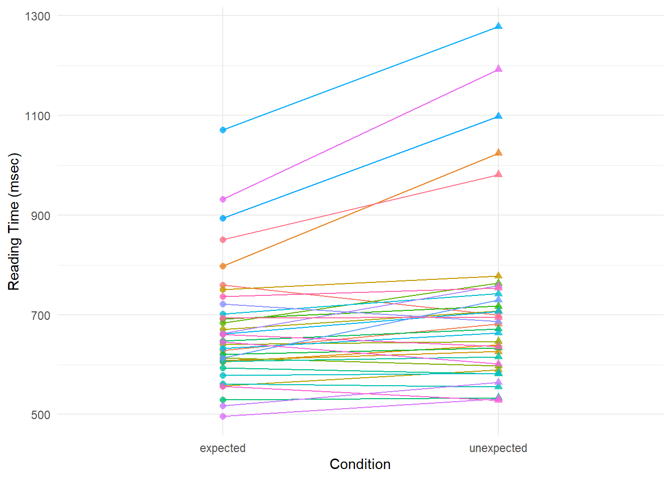
There’s a mix of ups and downs, and flat lines.
Would you guess from looking at all of these data that this effect would generalize?
- yes
- no
Thankfully we don’t have to just guess!
How likely is it that we would observe a difference at least this large (45 ms) if the null hypothesis were true - in this case, assuming the null hypothesis is that there is no reaction time difference between expected and unexpected articles? This is what a p-value measures. A p-value of .05 indicates that there is a 5% chance of observing an effect of at least this size even if the null hypothesis were true.
How to do Inferential Statistics
I’m showing you how to write the code for some statistical tests. This does not grant you a license to practice statistics, and does not provide you with any of the necessary background to know which tests to run and how to interpret them! Proceed with caution.
Preparing for Statistical Tests
In order to know which statistical tests are appropriate for your analysis, you need some statistical knowledge to work with the following important information.
- Your experimental design
- you should have a clear idea of what hypothesis is being tested
- statistical testing should be planned as part of the experimental design
- you should be able to write your statistical analysis before collecting any data!
- The nature of your data
- statistical tests are based on assumptions both about your design, AND your data
- to confirm that your chosen statistical tests are appropriate, you need to check for assumptions
- some can be checked with statistical “pre-tests”, some with visualizations
Choosing a statistical test is much more complex than following a decision tree or flowchart. It requires careful consideration of your theory, design, and data.
Preparing Data for Statistical Tests
The shape of your data will depend to some extent on what tests you are doing, but some general guidelines beyond the initial data cleaning and wrangling:
- check that variables are named correctly so you’re testing what you think you’re testing!
- model/run tests on unsummarized data, unless pre-summarization is a specific step in the analysis type you are conducting
- check that all variables are of the right type
- make sure that categorical variables are factors (or character), not numeric
- confirm dates are in the needed format
- confirm continuous numbers are the right numeric type
- check that the levels of factors are in the correct order and that contrasts are set as desired
- confirm units are consistent/as expected (temps in C or F? weight in kg or lb? population in thousands or millions?)
- evaluate missing data and adjust if needed
- transform, standardize, scale, and/or center variables as required
Coding Tests
We’re going to take the assumptions from the original Husband 2022 paper for our purposes, but simplify some of the analysis using a linear mixed effects model, like so:
A basic linear model would be generated using the lm() function:
#>
#> Call:
#> lm(formula = RT ~ expect, data = filter(rt.s.filt, rgn.fix ==
#>     0))
#>
#> Residuals:
#>    Min     1Q Median     3Q    Max
#> -603.8 -159.8  -66.9   62.4 3964.2
#>
#> Coefficients:
#>             Estimate Std. Error t value Pr(>|t|)
#> (Intercept)  694.419      5.423 128.041  < 2e-16 ***
#> expect1       44.803     10.847   4.131 3.72e-05 ***
#> ---
#> Signif. codes:  0 '***' 0.001 '**' 0.01 '*' 0.05 '.' 0.1 ' ' 1
#>
#> Residual standard error: 289.2 on 2842 degrees of freedom
#> Multiple R-squared:  0.005968,   Adjusted R-squared:  0.005618
#> F-statistic: 17.06 on 1 and 2842 DF,  p-value: 3.723e-05
The p-value is in the Pr(>|t|) column on the line with the fixed effect of expect1 (the effect of the “expected” level compared to the “unexpected” level). This is the probability of the t-statistic. Here is a simplified table output:
Closer to what is usually used in linguistic experimental work, we could also model the groupings of participants and items inherent in the data using a mixed effects model with lmer():
m_mixed <- lmer(RT ~ expect + (1 | Hash) + (1 + expect | item),
           data = filter(rt.s.filt, rgn.fix == 0))
summary(m_mixed)
#> Linear mixed model fit by REML. t-tests use Satterthwaite's method [
#> lmerModLmerTest]
#> Formula: RT ~ expect + (1 | Hash) + (1 + expect | item)
#> Data: filter(rt.s.filt, rgn.fix == 0)
#>
#> REML criterion at convergence: 39573.4
#>
#> Scaled residuals:
#> Min 1Q Median 3Q Max
#> -2.1107 -0.4872 -0.1664 0.2535 13.9999
#>
#> Random effects:
#> Groups Name Variance Std.Dev. Corr
#> item (Intercept) 908.5 30.14
#> expect1 3263.9 57.13 1.00
#> Hash (Intercept) 21297.0 145.93
#> Residual 61152.7 247.29
#> Number of obs: 2844, groups: item, 79; Hash, 36
#>
#> Fixed effects:
#> Estimate Std. Error df t value Pr(>|t|)
#> (Intercept) 694.17 24.99 36.29 27.774 < 2e-16 ***
#> expect1 43.99 11.30 91.85 3.893 0.000187 ***
#> ---
#> Signif. codes: 0 '***' 0.001 '**' 0.01 '*' 0.05 '.' 0.1 ' ' 1
#>
#> Correlation of Fixed Effects:
#> (Intr)
#> expect1 0.078
#> optimizer (nloptwrap) convergence code: 0 (OK)
#> boundary (singular) fit: see help('isSingular')You can read about the parallels between linear regression and other statistical tests from this site by Jonas Kristoffer Lindeløv.
What the lmer() version adds with “mixed effects” is the ability to model the groupings in the data over participants and items in the same model, as crossed effects. These are described as “random effects” and with lmer() have the syntax (1|random_effect_variable) (similar to the Error in aov()). Random slopes can be added as well as `(1 + random_slope | random_intercept). This is a very complex statistical topic that I will not even attempt to cover, but we can look at the same kind of model for the noun as well:
m_noun <- lmer(RT ~ expect + (1 | Hash) + (1 + expect | item),
           data = filter(rt.s.filt, rgn.fix == 1))
tbl_regression(m_noun, conf.int = FALSE)
Characteristic |
Beta |
p-value |
|---|---|---|
| expect | ||
| expected | 363 | <0.001 |
Often including all random slopes leads to errors and/or warnings. This is another very complex topic, but I will just point to the fact that some turn to Bayesian modelling to avoid these computational errors. A relatively easy package to use for Bayesian modelling that is similar to {lme4} is {brms}.
{brms} is a bit complex to setup as it is built on Bayesian analysis tools that are built with C++ code. There are instructions on setup out there, but the short version is it takes more than just installing the package itself. I’m not going to show you the relevant code because it’s not something you can just easily try out, or even interpret. Bayesian modelling has its own foundations and assumptions, and you would need to dedicate some serious time to learning it, beyond learning linear mixed effects modelling.
Next Steps in Statistics
If you don’t know any statistics
Really you should take at least an introductory statistics course to learn the foundations about distributions and probability. It’s easier to do this while you’re in college and already paying tuition! However, if you need to learn it on your own, there are some resources that are linguistics-oriented for the beginner.
How to do Linguistics with R by Natalia Levshina is a good R-based introduction that takes you through the basics of statistics, including analyses like t-tests and ANOVAs. It also covers a very broad range of model types. It is a bit outdated when it comes to the package used for mixed effects modelling (it came out before {lmer4} was released), but gives a good broad foundation, and you can figure out the {lme4} details from other sources. You probably will not want to work through this entire book, but start from the beginning and then learn the types of models that are relevant for the work you are doing.
Analyzing Linguistics Data by R.H. Baayen is also a good text, but it is even more outdated now unfortunately.
The PsyTeachR Analysis book is psychology-focused, but in a way that is very relevant to linguistic research as well. This book goes through statistics basics, like the Levshina book, but is very current and freely available online.
If you know some (general) statistics
If you have taken courses like STATS 250 or even some higher-level statistics courses, you (should) know the foundations of statistics, but likely do not know about the analyses typically used in linguistics. These approaches are usually not taught in general coursework, but rather in linguistics- or psychology-specific courses. For most types of linguistic work, you need to learn linear mixed effects models, and possibly generalized linear mixed effects. There is a ton of jargon overlap and confusion in this area, but these are sometimes also referred to as hierarchical modelling or hierarchical regression. The only UM course I’m aware of at the undergraduate level which covers these models is PSYCH 463, which requires previous stats knowledge (of regression).
Joe Fruehwald’s Statistical Modelling with R Course is a fantastic quick starter on the basics of linear mixed effects models, and what their purpose is. You can quickly read/skim the early chapters on data wrangling and learn more about the statistics from meetings 5-8.
Statistics for Linguistics by Bodo Winter is a great book for quickly getting familiar with (generalized) mixed effects modelling, though it really skims over some foundational statistical concepts. It is probably the most comprehensive “quick start” and what I usually have students in my lab work through, given I can help them with the basics as needed. You may feel a bit unmoored doing analysis on your own if you only read this and still don’t know what a t-test is, or how ANOVAs work. It is available as an e-book through the library.
PsyTeachR’s Learning Statistical Models Through Simulation in R is a great walkthrough from the basic linear model into mixed-effects models, including generalized models.
R for Prediction and Machine Learning
Some of you have inquired about how these skills can be used in a “business” context. Many businesses use experiments (such as A/B testing websites) and surveys which require data cleaning/wrangling and statistical tests similar to what we have been working on. Businesses also frequently want to do predictive modeling, which uses similar methods as inferential statistical tests to predict future datapoints about all kinds of things! Here is a case study using hotel bookings that is demonstrated using the {tidymodels} suite of tools. {tidymodels} helps with running many models and comparing their output.
Any direction you go with data, you will use the foundational principles of data wrangling and report generation that we have discussed in class. What goes in the middle of that sandwich is very domain specific and requires an understanding of the field itself (e.g., the hotel business, or psycholinguistics), the statistical tools relevant for that field, and the most useful technical tools to execute those analyses.
Older episodes (go back to the beginning) of the Not So Standard Deviations podcast have some interesting discussions about data analysis and data science in the context of both academia (primarily from Roger Peng) and business (primarily from Hilary Parker).
There are also a lot of RStudio::conf/Posit::conf talks about different business/industry topics that you can find on YouTube or the Posit website.